Flow and Diffusion models Part 2 - Fokker-Planck

Lecture 2 This is the most mathmatical chanllenging part of the lecture, but also covers all the missing knowledge I would like to learn, like Langevin and Fokker-Planck

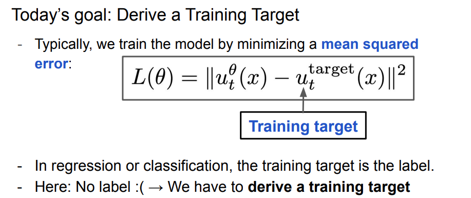
1 Training goal

Review two models we learned so far 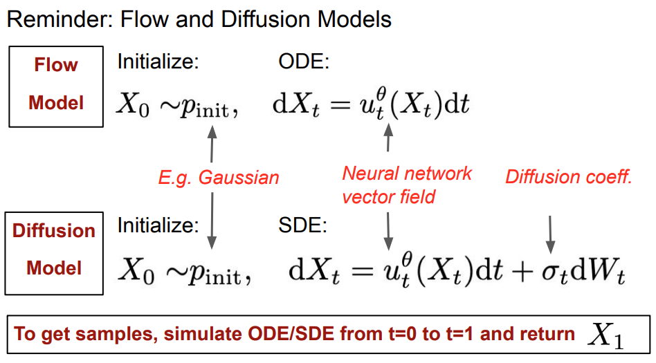Learning goal is to find the formula for the target vector field such taht corresponding ODE/SDE convert $p_init$ to $p_data$

Two key concepts

• conditional: per single data point
• marginal: across distribution of all data points

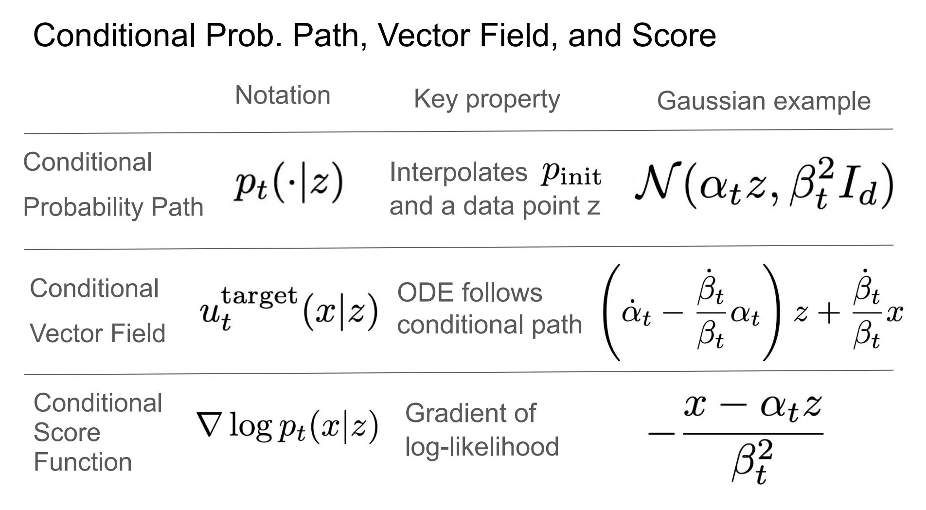
2 Probability Path

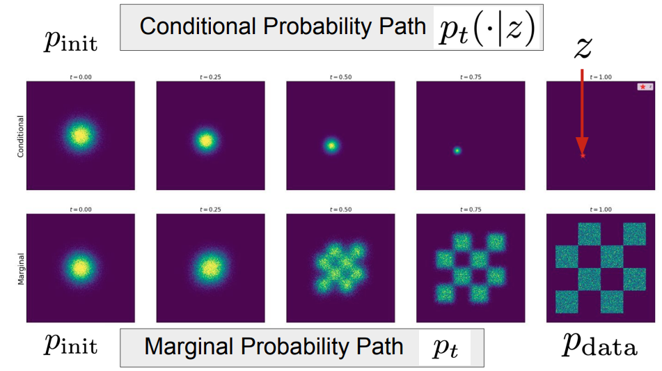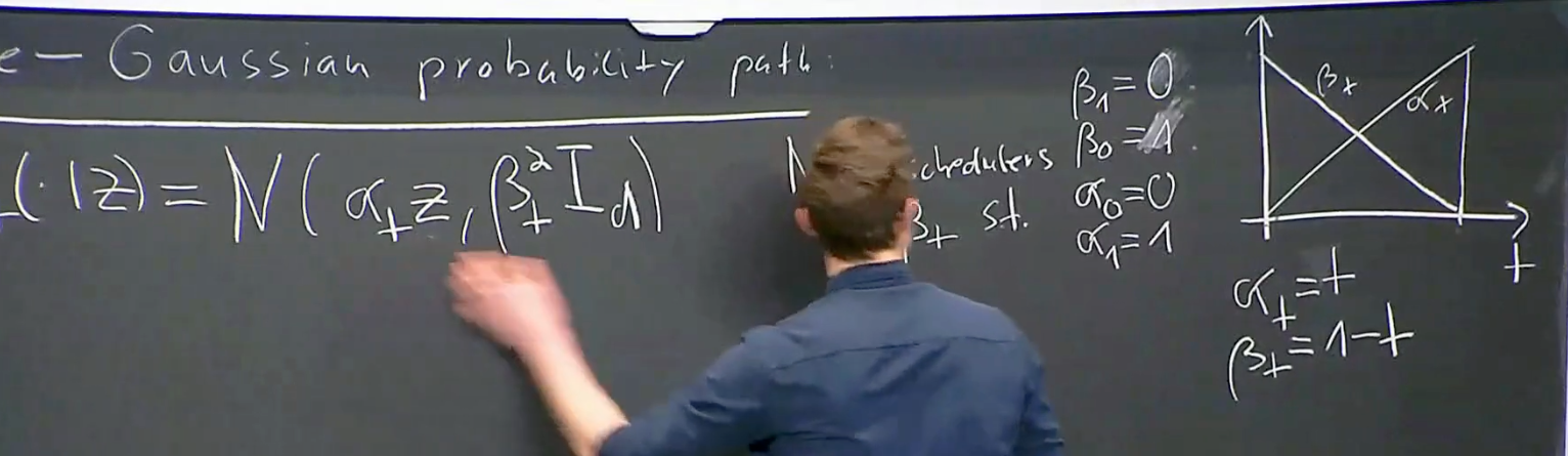
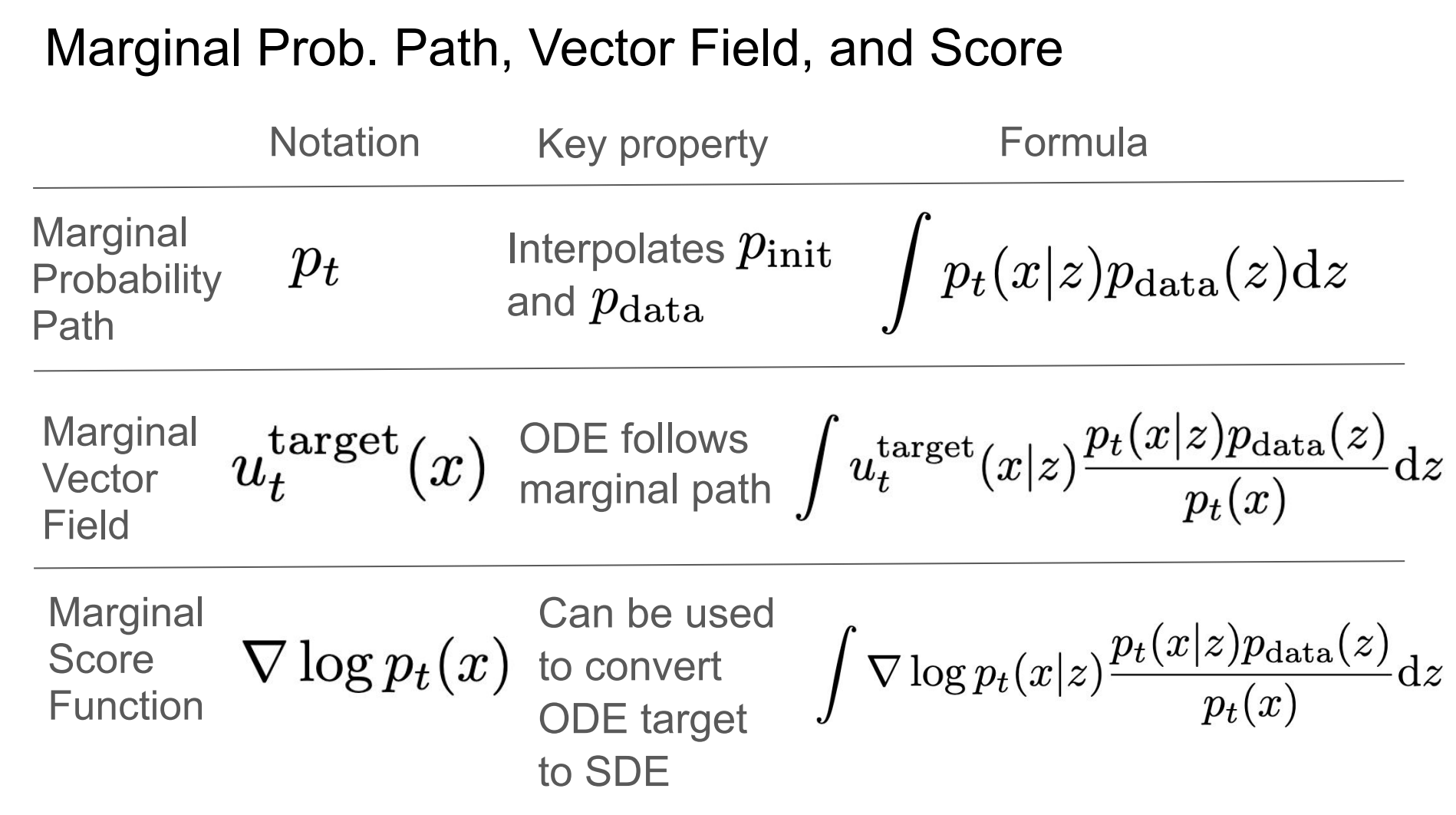
For conditional probability path We have a example of Gaussian prob path with noise schedule s.t For marginal probablity path, this is a bit hard to digest. The key idea is to understand probability path as a trajectory in the space of distributions. 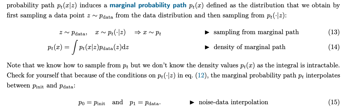The density $p_t(x)$ is unkonw because the integral is intractable.

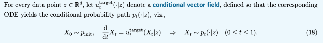
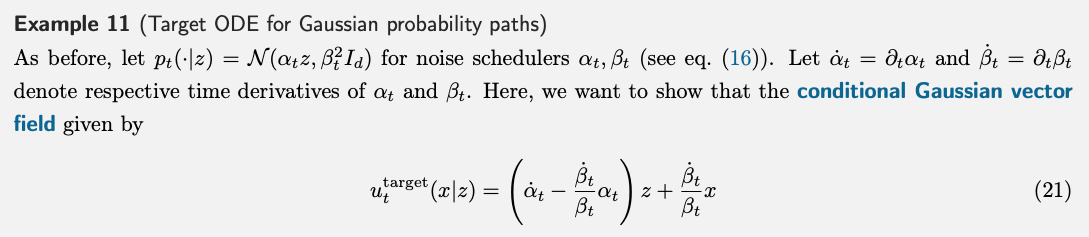
3 Vector Field

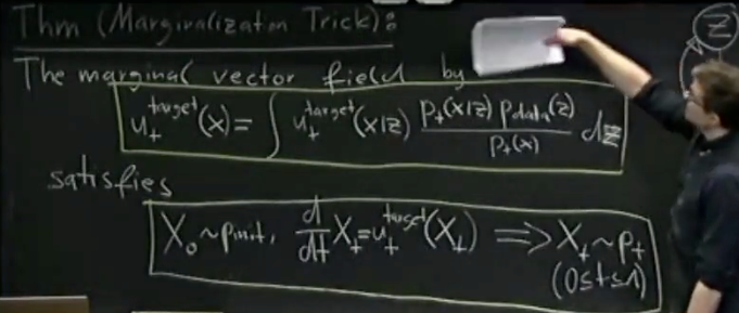
If we simulate a ODE with a conditional vector field, then any state on the trajectory is following conditional probabilty path. The Gaussian example is given by The Marginalization Trick, which can be approved by Continity equation,

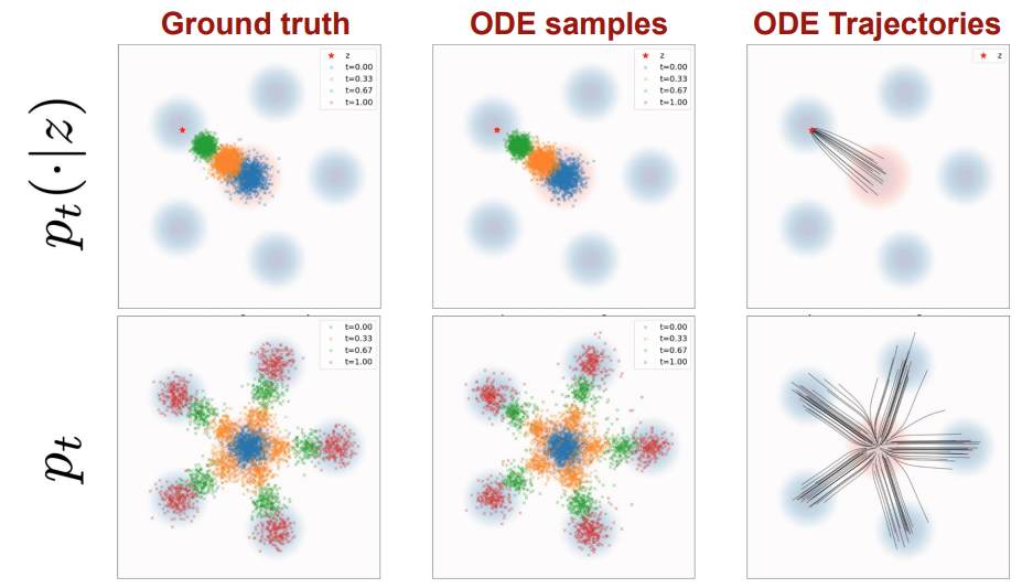
Here is the comparison of these two under ODE samples

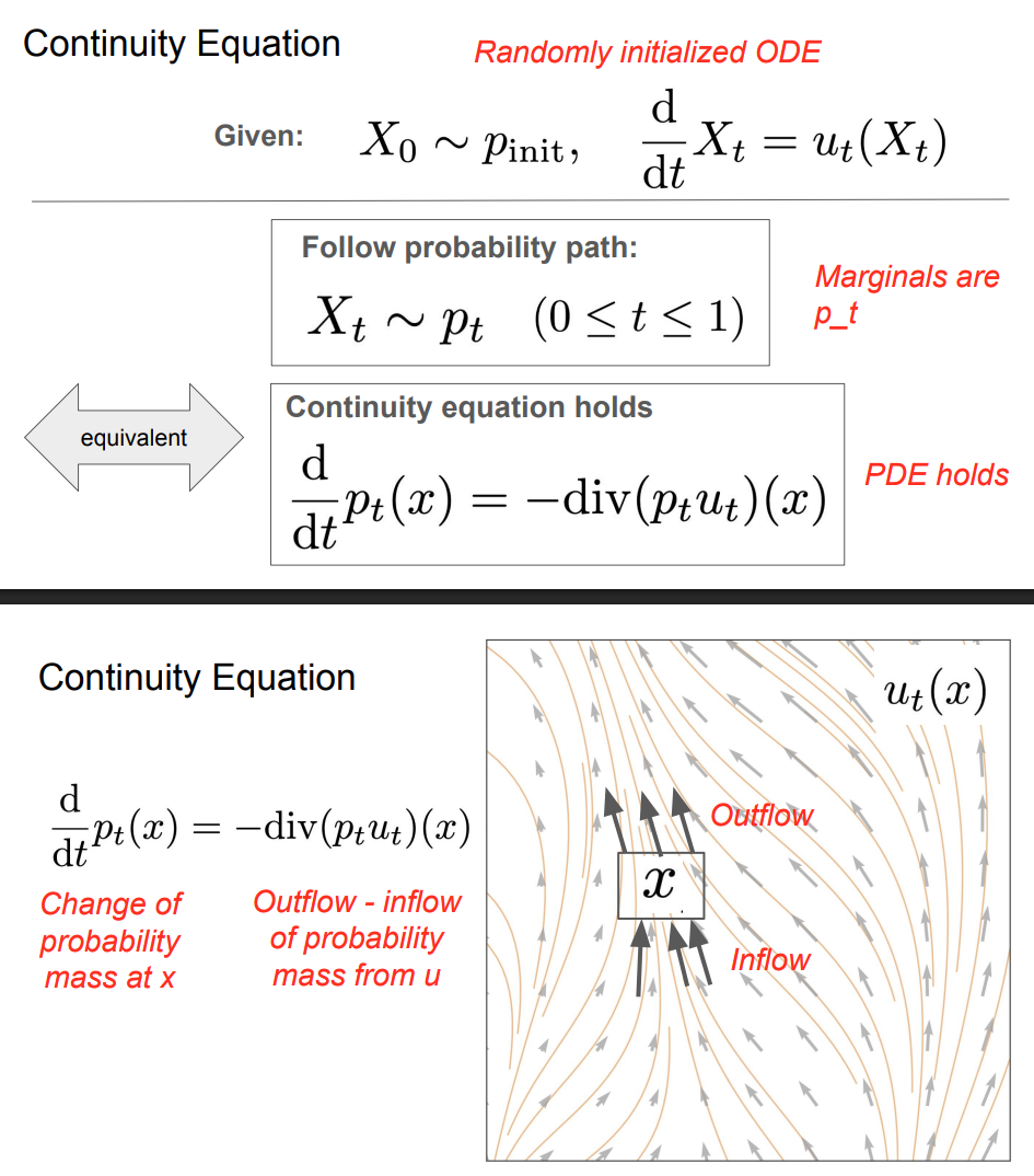
4 Continuity Equation

CE can be interpreated by the conservation of probability mass. From this equation, we can derive the marginalization trick

5 Score Function

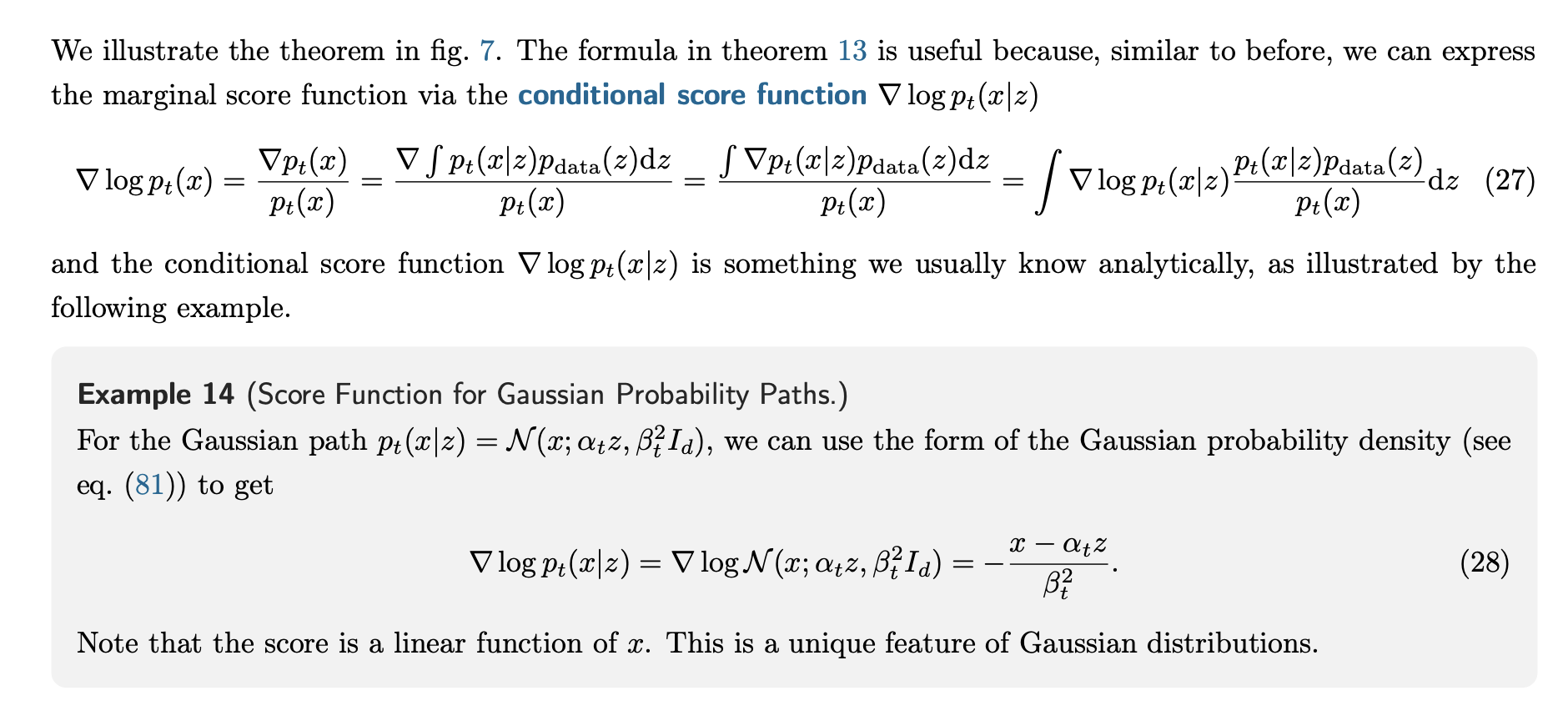
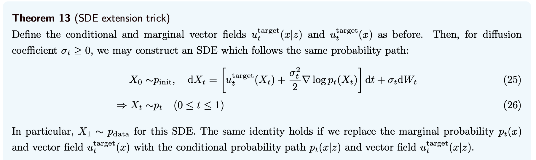
Score function is defined as the grad of the log of the density. and marginal score can be get from conditional score Now we do SDE extension trick. When there is diffusion terms added in the SDE, the vector field should be adjusted accordingly, so the same condition holds as in the marginalization trick.

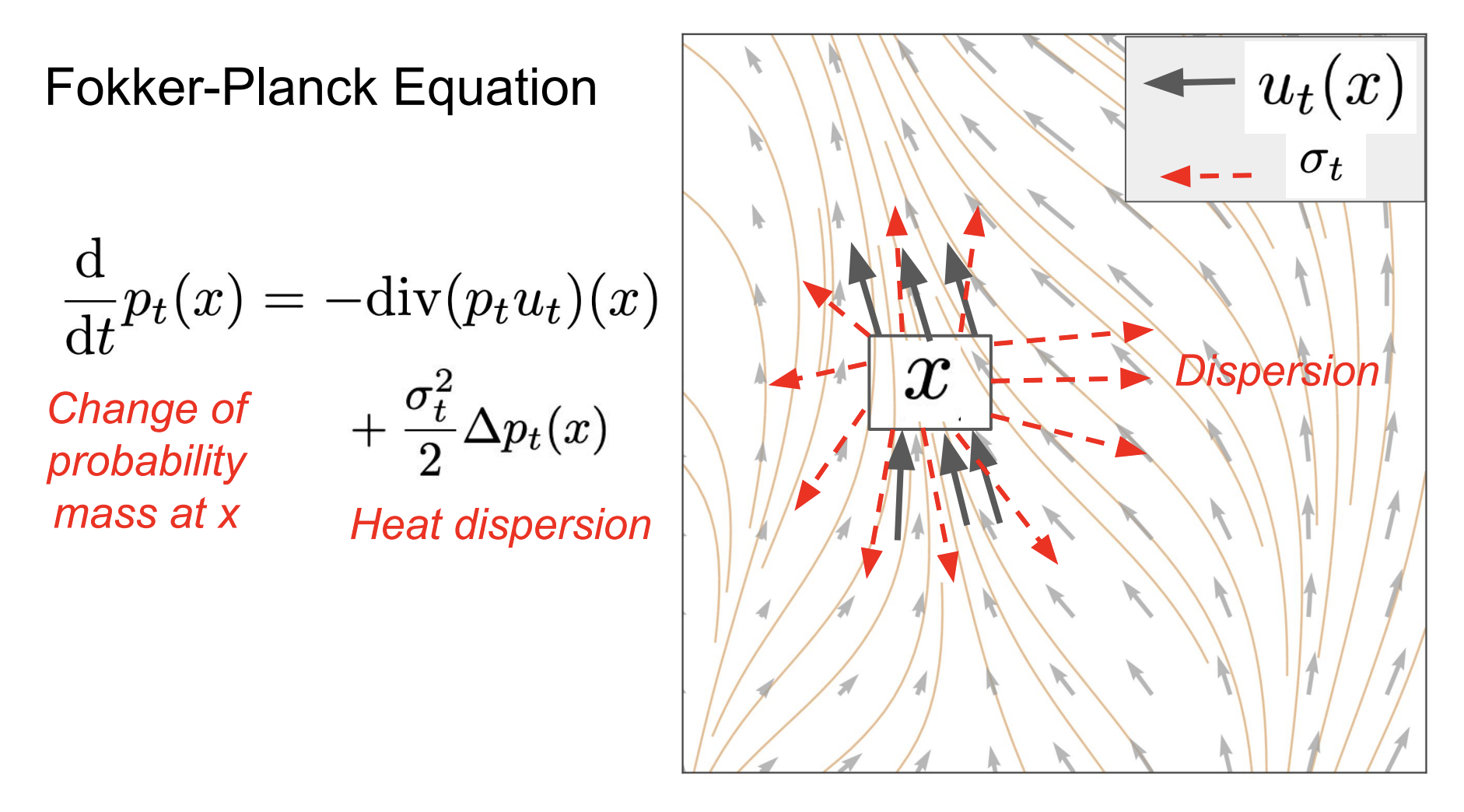
6 Fokker-Planck Equation

SDE extension trick can be approved by Fokker-Planck equation, which is the SDE version of the continuity equation. 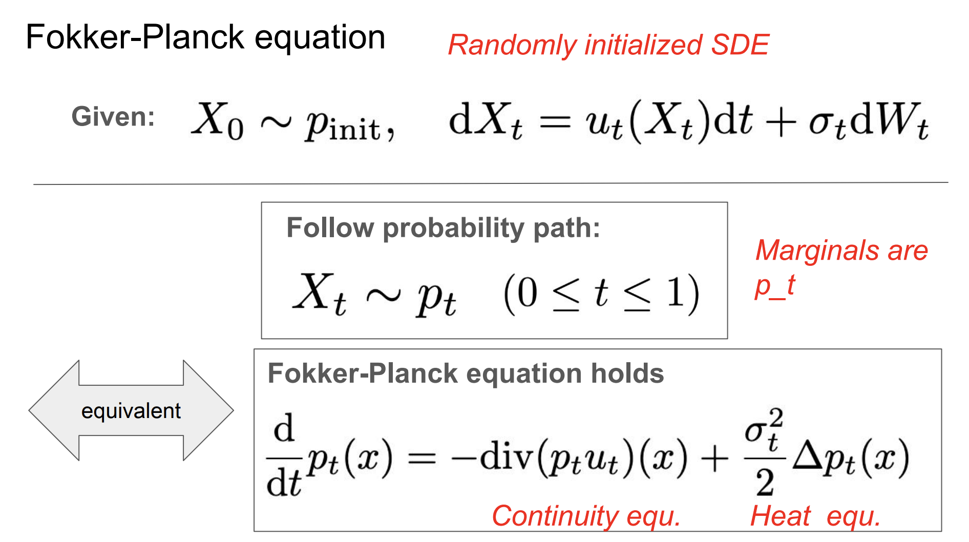And the physical interpretation is adding heat dispersion The proof of SDE extension is a bit confusing to me. It actually starts from continuity equation, and then satisfied with Fokker-Planck equation…

7 Summary