Flow and Diffusion models Lab 2-1 - Gaussian Probability Path w Flow matching

1 Gaussian Conditional Probability Path

Gaussian conditional probability path is given by \(p_t(x|z) = N(x;\alpha_t z,\beta_t^2 I_d),\quad\quad\quad p_{\text{simple}}=N(0,I_d),\) where $\alpha_t: [0,1] \to \mathbb{R}$ and $\beta_t: [0,1] \to \mathbb{R}$ are monotonic, continuously differentiable functions satisfying $\alpha_1 = \beta_0 = 1$ and $\alpha_0 = \beta_1 = 0$.
In other words, this implies that $p_1(x|z) = \delta_z$ and $p_0(x|z) = N(0, I_d)$ is a unit Gaussian.
and we can use $\alpha_t = t$ and $\beta_t = \sqrt{1-t}$

class LinearAlpha(Alpha):
    """
    Implements alpha_t = t
    """
    def __call__(self, t: torch.Tensor) -> torch.Tensor:
        return t
    def dt(self, t: torch.Tensor) -> torch.Tensor:
        return torch.ones_like(t)
class SquareRootBeta(Beta):
    """
    Implements beta_t = squareroot(1-t)
    """
    def __call__(self, t: torch.Tensor) -> torch.Tensor:
        return torch.sqrt(1-t)
    def dt(self, t: torch.Tensor) -> torch.Tensor:
        return - 0.5 / (torch.sqrt(1 - t) + 1e-4)

Now we can have the groundtruth of the GCPP

class GaussianConditionalProbabilityPath(ConditionalProbabilityPath):
    def __init__(self, p_data: Sampleable, alpha: Alpha, beta: Beta):
        p_simple = Gaussian.isotropic(p_data.dim, 1.0)
        super().__init__(p_simple, p_data)
        self.alpha = alpha
        self.beta = beta

    def sample_conditioning_variable(self, num_samples: int) -> torch.Tensor:
        """
        Samples the conditioning variable z ~ p_data(x)
        Args:
            - num_samples: the number of samples
        Returns:
            - z: samples from p(z), (num_samples, dim)
        """
        return self.p_data.sample(num_samples)
    
    def sample_conditional_path(self, z: torch.Tensor, t: torch.Tensor) -> torch.Tensor:
        """
        Samples from the conditional distribution p_t(x|z) = N(alpha_t * z, beta_t**2 * I_d)
        Args:
            - z: conditioning variable (num_samples, dim)
            - t: time (num_samples, 1)
        Returns:
            - x: samples from p_t(x|z), (num_samples, dim)
        """
        return self.alpha(t) * z + self.beta(t) * torch.randn_like(z)

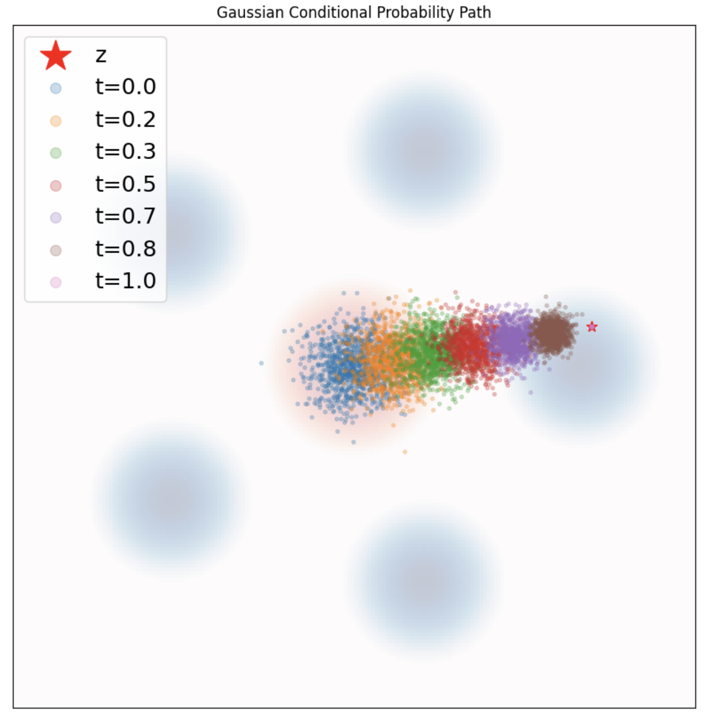
To show the probality path, plot samples

for t in ts:
    zz = z.expand(num_samples, 2)
    tt = t.unsqueeze(0).expand(num_samples, 1) # (samples, 1)
    samples = path.sample_conditional_path(zz, tt) # (samples, 2)

2 Flowing Matching using Conditional Vector Field

Analytically, we know that the conditional vector field $u_t(x|z)$ is given by \(u_t(x|z) = \left(\dot{\alpha}_t-\frac{\dot{\beta}_t}{\beta_t}\alpha_t\right)z+\frac{\dot{\beta}_t}{\beta_t}x.\)

class GaussianConditionalProbabilityPath(ConditionalProbabilityPath):
  ...
  def conditional_vector_field(self, x: torch.Tensor, z: torch.Tensor, t: torch.Tensor) -> torch.Tensor:
        """
        Evaluates the conditional vector field u_t(x|z)
        Note: Only defined on t in [0,1)
        Args:
            - x: position variable (num_samples, dim)
            - z: conditioning variable (num_samples, dim)
            - t: time (num_samples, 1)
        Returns:
            - conditional_vector_field: conditional vector field (num_samples, dim)
        """ 
        alpha_t = self.alpha(t) # (num_samples, 1)
        beta_t = self.beta(t) # (num_samples, 1)
        dt_alpha_t = self.alpha.dt(t) # (num_samples, 1)
        dt_beta_t = self.beta.dt(t) # (num_samples, 1)
        return (dt_alpha_t - dt_beta_t / beta_t * alpha_t) * z + dt_beta_t / beta_t * x   

Define the ODE $d X_t = u_t(X_t|z)dt, \quad X_0 = x_0 \sim p_{\text{simple}}.$. Drift coefficient is just the vector field.

class ConditionalVectorFieldODE(ODE):
    def __init__(self, path: ConditionalProbabilityPath, z: torch.Tensor):
        super().__init__()
        self.path = path
        self.z = z
    def drift_coefficient(self, x: torch.Tensor, t: torch.Tensor) -> torch.Tensor:
        bs = x.shape[0]
        z = self.z.expand(bs, *self.z.shape[1:])
        return self.path.conditional_vector_field(x,z,t)

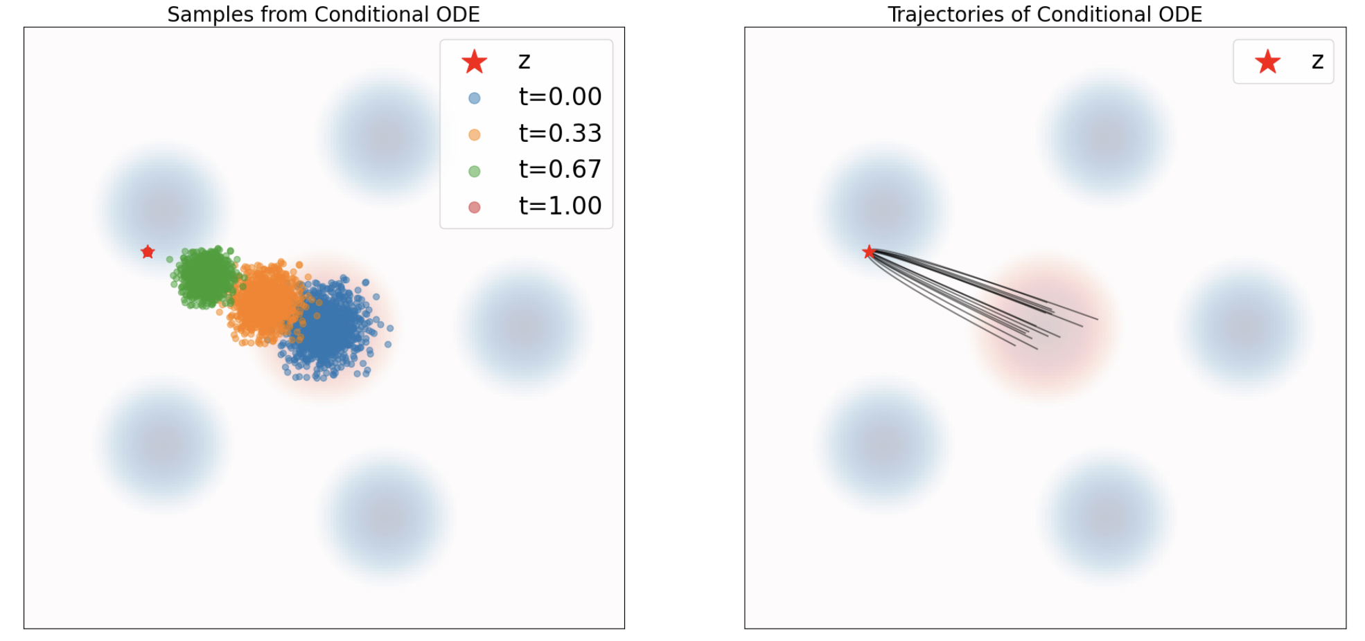
Extract every n-th step from xts get the 1st figure and show all xts get the 2nd figure

ode = ConditionalVectorFieldODE(path, z)
simulator = EulerSimulator(ode)
x0 = path.p_simple.sample(num_samples) # (num_samples, 2)
ts = torch.linspace(0.0, 1.0, num_timesteps).view(1,-1,1).expand(num_samples,-1,1).to(device) # (num_samples, nts, 1)
xts = simulator.simulate_with_trajectory(x0, ts) # (bs, nts, dim)

3 Training for Flow matching

Due to the marginal vector field can be get from weighted conditional vector field, the loss function based on marginal vector field equals to a constant, plus loss function of conditional vector field. So we can train based on conditional vector field \(\mathcal{L}_{CFM}(\theta) = \,\mathbb{E}_{t \in \mathcal{U}[0,1), z \sim p(z), x \sim p_t(x|z)} {\lVert u_t^{\theta}(x) - u_t^{\text{ref}}(x|z)\rVert^2}\) using a Monte-Carlo estimate of the form \(\frac{1}{N}\sum_{i=1}^N {\lVert u_{t_i}^{\theta}(x_i) - u_{t_i}^{\text{ref}}(x_i|z_i)\rVert^2}, \quad \quad \quad \forall i\in[1, \dots, N]: {\,z_i \sim p_{\text{data}},\, t_i \sim \mathcal{U}[0,1),\, x_i \sim p_t(\cdot | z_i)}.\) Here is how we sample

• z is sampled from p_data
• t is sampled from torch.rand
• x is sampled from path.sample_conditional_path(z, t), same as groundtruth
• u_ref is get from path.conditional_vector_field(x,z,t), same as drift coeff used with in simulate_with_trajectory

  class ConditionalFlowMatchingTrainer(Trainer):
    def __init__(self, path: ConditionalProbabilityPath, model: MLPVectorField, **kwargs):
        super().__init__(model, **kwargs)
        self.path = path
    def get_train_loss(self, batch_size: int) -> torch.Tensor:
        z = self.path.p_data.sample(batch_size) # (bs, dim)
        t = torch.rand(batch_size,1).to(z) # (bs, 1)
        x = self.path.sample_conditional_path(z,t) # (bs, dim)
        ut_theta = self.model(x,t) # (bs, dim)
        ut_ref = self.path.conditional_vector_field(x,z,t) # (bs, dim)
        error = torch.sum(torch.square(ut_theta - ut_ref), dim=-1) # (bs,)
        return torch.mean(error)
  

  Train the model with MLP, pretty standard, and now you have an ODE, which directly use the trained vector field as drift coeff. ( Before we use vector field from the probability path )

  class LearnedVectorFieldODE(ODE):
    def __init__(self, net: MLPVectorField):
        self.net = net
    def drift_coefficient(self, x: torch.Tensor, t: torch.Tensor) -> torch.Tensor:
        return self.net(x, t)
  

  Now we can plot out the simulated path xts. Be aware that this marginal probability path, so data are spread into all possible distributions, NOT only converged into one single sample z as in conditional probability path.

  ode = LearnedVectorFieldODE(flow_model)
  # compare to ode = onditionalVectorFieldODE(path, z)
  simulator = EulerSimulator(ode)
  x0 = path.p_simple.sample(num_samples) # (num_samples, 2)
  ts = torch.linspace(0.0, 1.0, num_timesteps).view(1,-1,1).expand(num_samples,-1,1).to(device) # (num_samples, nts, 1)
  xts = simulator.simulate_with_trajectory(x0, ts) # (bs, nts, dim)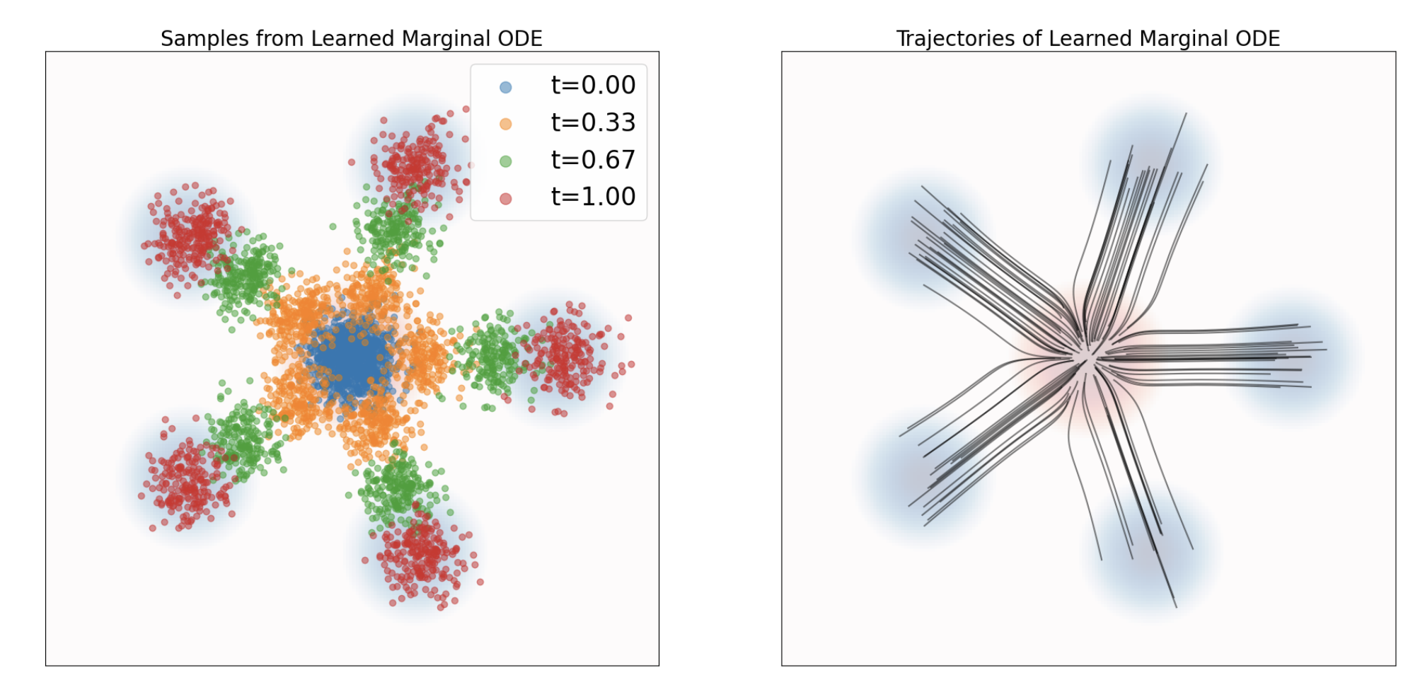
  

  

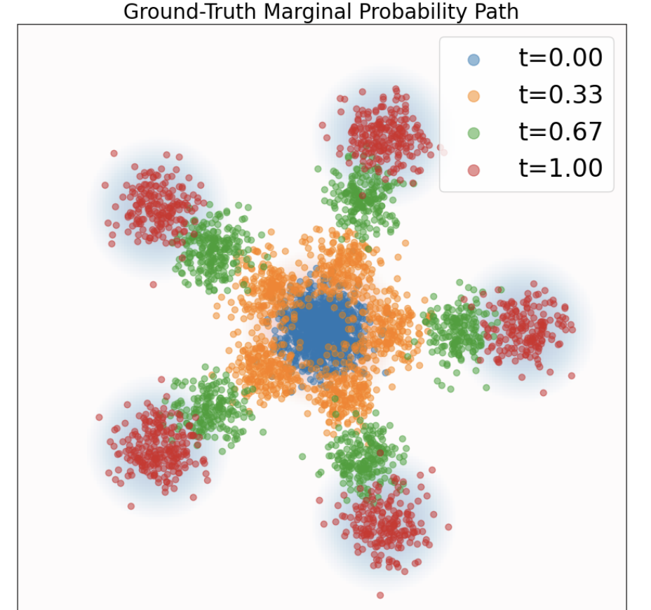
We can also plot out the groundtruth, which is directly get from sample_marginal_path. The implementation is actually still use sample_conditional_path but with num_samples output

class ConditionalProbabilityPath(torch.nn.Module, ABC):
    ...
    def sample_marginal_path(self, t: torch.Tensor) -> torch.Tensor:
        """
        Samples from the marginal distribution p_t(x) = p_t(x|z) p(z)
        Args:
            - t: time (num_samples, 1)
        Returns:
            - x: samples from p_t(x), (num_samples, dim)
        """
        num_samples = t.shape[0]
        # Sample conditioning variable z ~ p(z)
        z = self.sample_conditioning_variable(num_samples) # (num_samples, dim)
        # Sample conditional probability path x ~ p_t(x|z)
        x = self.sample_conditional_path(z, t) # (num_samples, dim)
        return x