Diffusion Models

The original motivation of this tech blog was to understand diffusion models. It’s such a beautify algorithm that I spent lots of time reading from

1. Lilian’s blogs(Great summary of diffusion models. I feel this blog is Lilian’s own study notes, in a high-bar quality.)
2. Assembly AI’s blogs (Shout out to Ryan O’Connor, who writes great blogs which has nothing to do Assemly AI’s business :P)
3. 苏神’s blogs (His blogs are totally in another level, from insightful math perspectives)

One year later, I decided to review them and record it down here. I also found couple of good resources recently and mainly use them as the contents here.

1. Umar’s youtube
2. Steins’ explanations

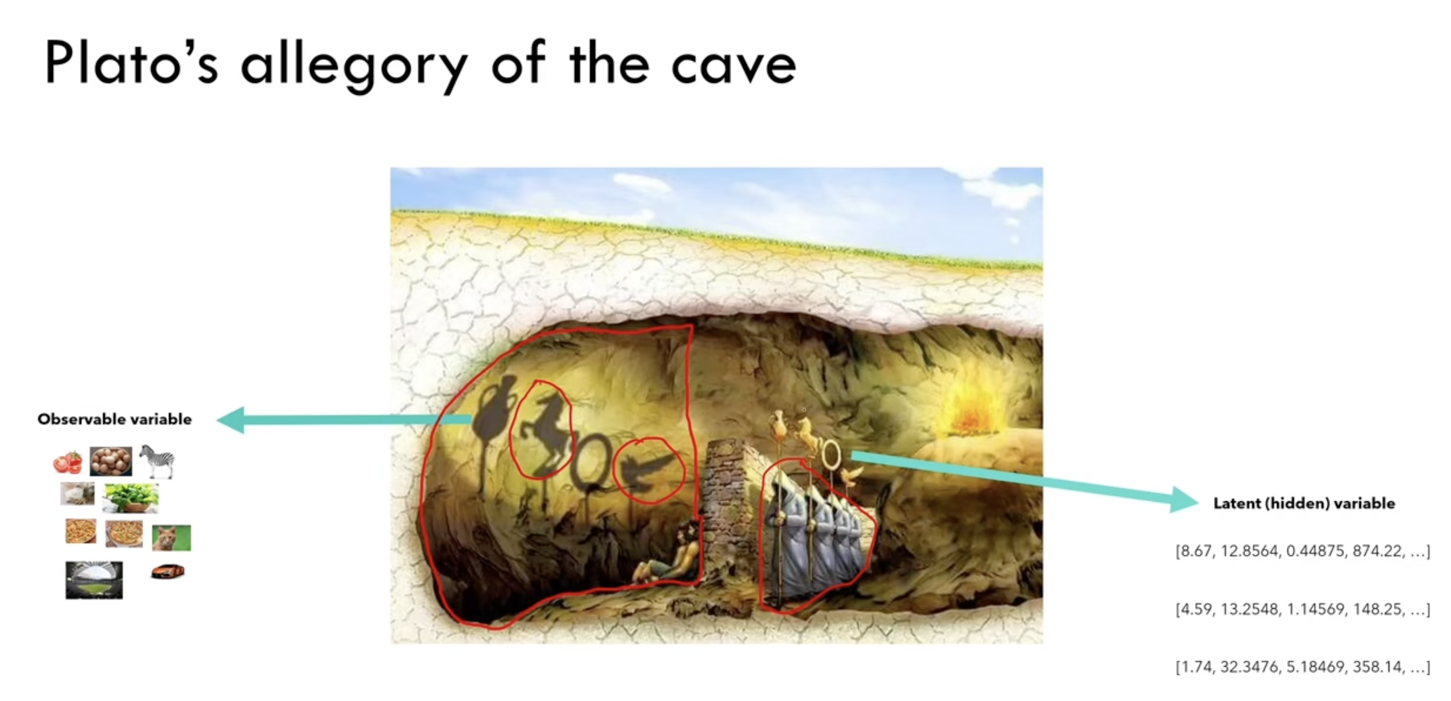
Let’s start w Platot’s allegory of the cave, a very unique analogy from Umar’s video. So we human are just chained in a cave?

0 Reparameterization trick

First thing to demystify is re-parameterization trick. Frankly speaking I never understand the figure which is used everywhere to explain the trick. 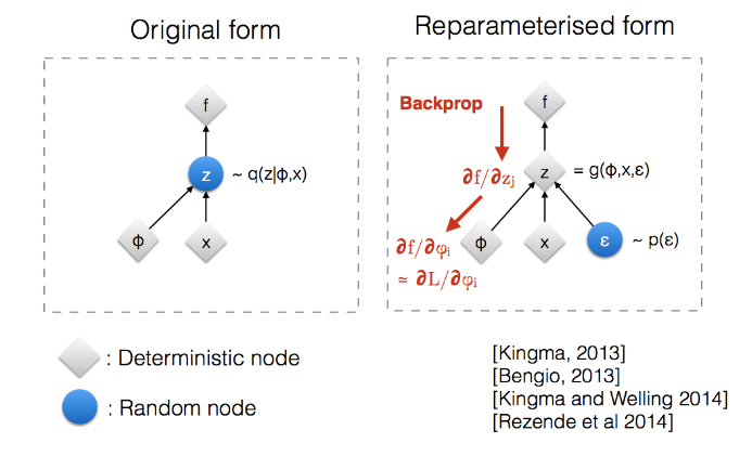But mathmatically, it’s just \(\mathit{if}\ \ z \sim \mathcal{N}(\mu, \sigma^2)\ \mathit{then}\\ z=\mu+ \sigma\epsilon\ \ \ \mathit{where}\ \epsilon \sim \mathcal{N}(0,1)\)

1 Forward Process

Adding noise in $T$ steps and step sizes are controlled by a vairance schedule ${\beta_t\in(0,1)}^T_{t=1}$ 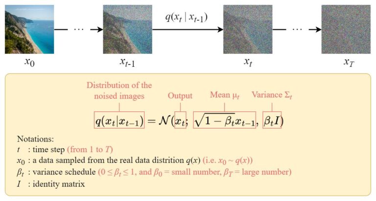Based on the re-parameterization trick, it gives \(x_t=\sqrt{1-\beta_t}\ x_{t-1}+\sqrt{\beta_t}\ \epsilon_{t-1} \ \ \ (1)\) A closed-form formular can be derived as
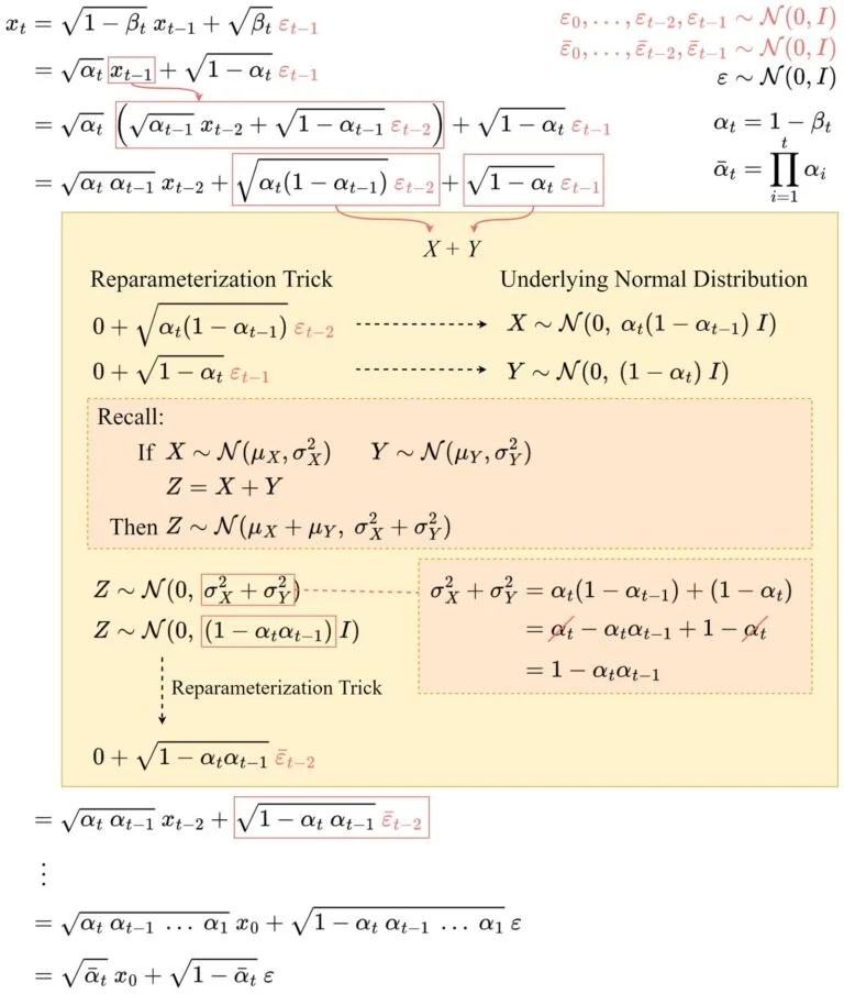
All basic statistical calculations, finally gives you the formulat that you can directly sample $x_t$ at any time step \(x_t=\sqrt{\bar\alpha_t}\ x_0+\sqrt{1-\bar\alpha_t}\ \epsilon\ \ \ (2)\) Now you can see where we get the formular in the training algorithm

2 Reverse Process

The direct reverse process is intractable, so we train a neural network $p_{\theta}(x_{t-1}\mid x_t)$ to approximate the process $q(x_{t-1}\mid{x_t})$.

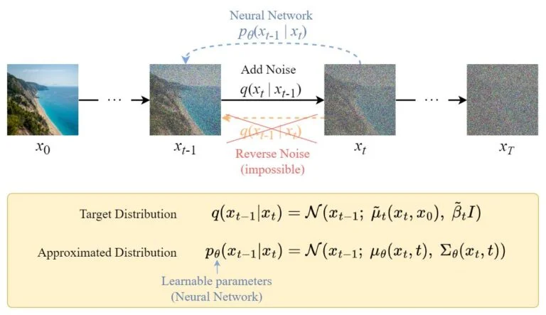
For simplicity, we assume multivariate Gaussian is a product of independent gaussians with identical variance, and futhur set these variances to be equivalent to our forward process variance schedule.\(\Sigma_{\theta}(x_t,t) = \sigma_t^2\mathrm{I} \\where\ \sigma_t^2=\beta_t\)

To get the mean, we can derive from the $q(x_{t-1}\mid x_t)$ All these steps below are based on formular 1 and 2 to write out the explicity form of normal distribution. I once gave them to my daughter and she worked it out 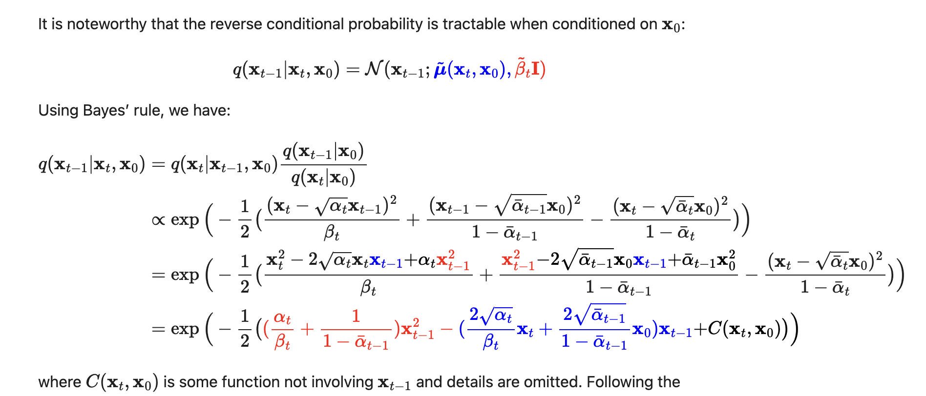Following the defination of standard Gaussian density function, the mean and variance can be parameterized as follows

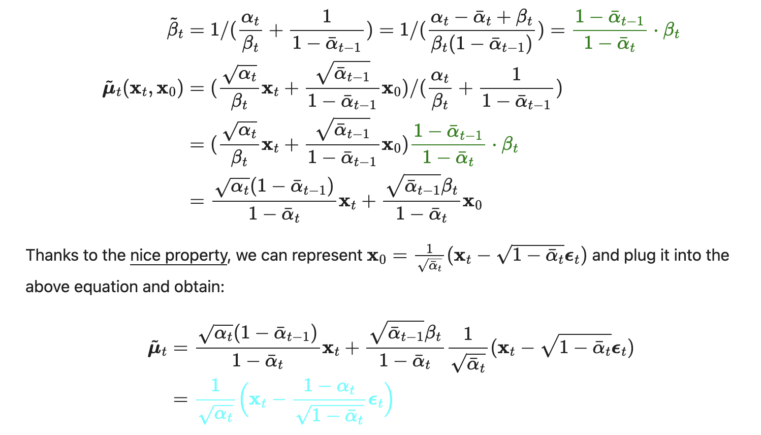
These formulas are used in the sampling algorithm.

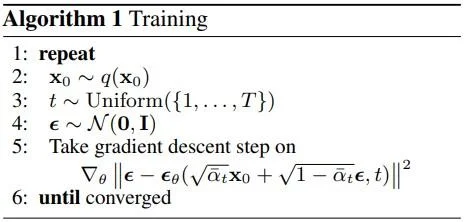
3 Training

The network is used to predict noise at time step $t$, with input of the noised image $x_t$ and $t$.

The lose function will be explained in my next note, which is the most challenging part of this algorithm.

# Generate noise, one for each image in the batch
epsilons = torch.randn(batch.shape, device=self.device)
# ts[i] is the randome time step for the i_th batch image
# ts = torch.randint(0, self.t_range, [batch.shape[0]],...) 
for i in range(len(ts)):
    a_hat = self.alpha_bar(ts[i])
    noise_imgs.append(
        (math.sqrt(a_hat) * batch[i]) + (math.sqrt(1 - a_hat) * epsilons[i])
    )
noise_imgs = torch.stack(noise_imgs, dim=0)
# Run the noisy images through the U-Net, to get the predicted noise
e_hat = self.forward(noise_imgs, ts)
# Calculate the loss, that is, the MSE between the predicted noise and the actual noise
loss = nn.functional.mse_loss(
    e_hat.reshape(-1, self.in_size), epsilons.reshape(-1, self.in_size)
)

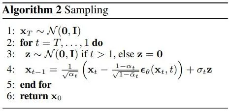
4 Sampling

With the model trained, following steps below we can denoise the image step by step from a random noise.

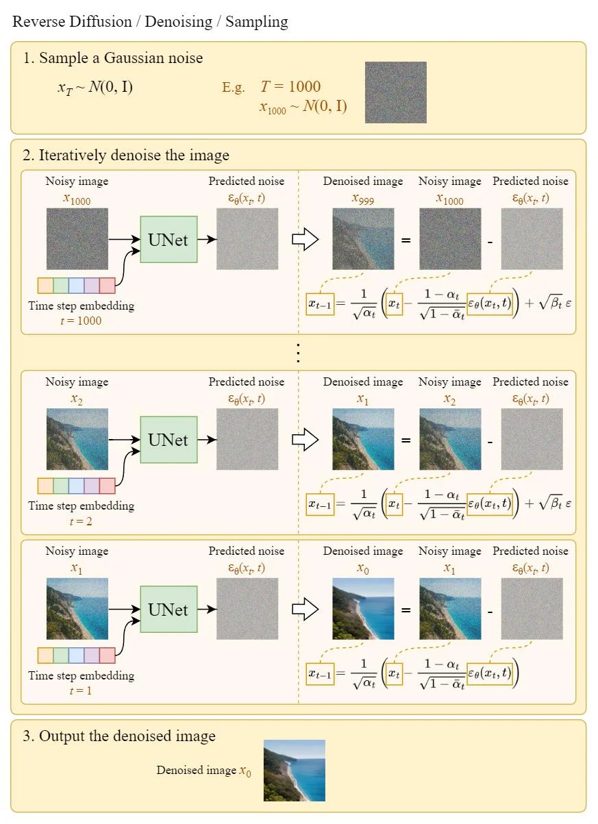
Here are the steps in code.

# Get the predicted noise from the U-Net
e_hat = self.forward(x, t.view(1).repeat(x.shape[0]))
# Perform the denoising step to take the image from t to t-1
pre_scale = 1 / math.sqrt(self.alpha(t))
e_scale = (1 - self.alpha(t)) / math.sqrt(1 - self.alpha_bar(t))
post_sigma = math.sqrt(self.beta(t)) * z
x = pre_scale * (x - e_scale * e_hat) + post_sigma

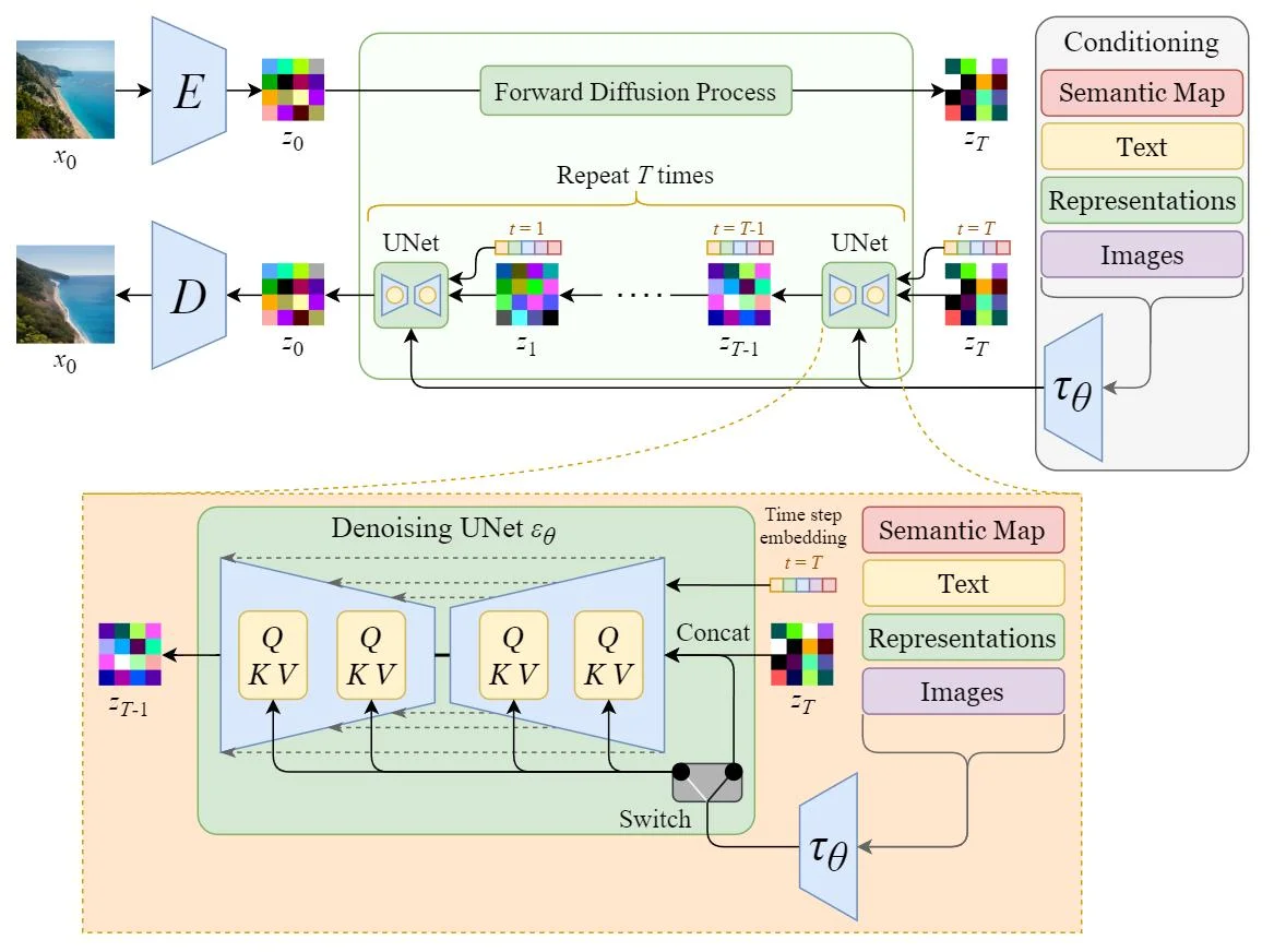
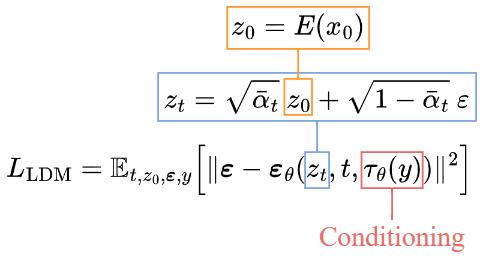
5 Stable Diffusion

The vallina Diffusion is adding noise the the original images. “Latent Diffusion Model” (LDM). As its name points out, the Diffusion process happens in the latent space, which is faster. 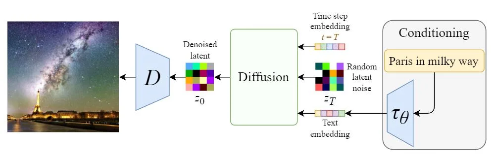Text embedding can be added to have the image generation conditioned on the title. So the high level algo is showed below with $E$ as the encoder for the image. The sampling is conditioned as well, with a decode at the end.