Andrej Karpathy-MLP

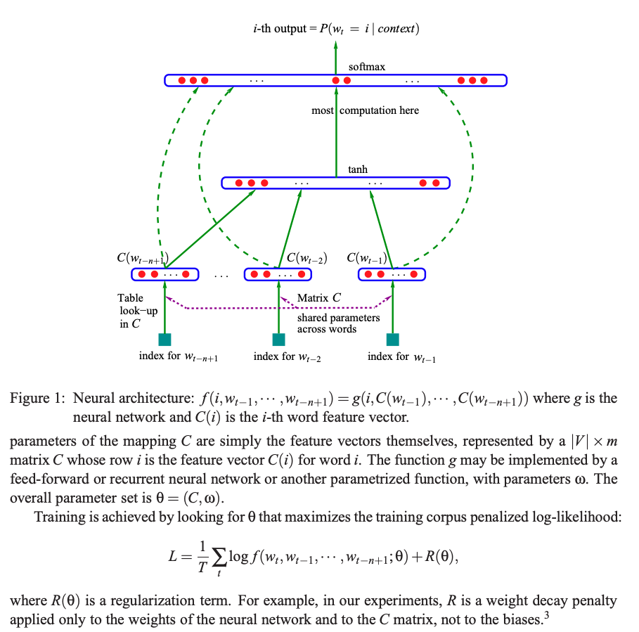
It’s based on Bengio’s paper on MLP, A Neural Probabilistic Language Model in 2003.

$C$ is embedding matrix 17,000 x emb_size. Last layer has 17,000 neurons, for 17,000 words. and the middle layer’s neuron number is h-para, say 100. If we look back 3 words (n=3), the first layer $W$ has size (3*emb_size, 100) (Ignore the green dotted lines)

1 Data Preparation

• Context window

  # for each word 2
  block_size = 3
  context = [0] * block_size
  for ch in w + '.':
    ix = stoi[ch]
    X.append(context)
    Y.append(ix)
    context = context[1:] + [ix] # crop and append
  X = torch.tensor(X) # total_ch x block_size
  Y = torch.tensor(Y) # total_ch
  

• Embedding table C

  # embedding table, #_embed x len_embed
  # Set len_embed = 2
  C = torch.randn((27, 2))
  # Each value of X is within 0~27 
  emb = C[X]
  # So the embed size is X shape appended by 2
  emb.shape # X.shape + [2] -> (total_ch,3,2) 
  

• Embed words concatentations We need convert (chx3x2)->(chx6)

  # Direct cat, on dim 1 (for chx2)
  torch.cat([emb[:,0,:],emb[:,1,:],emb[:,2,:]], 1)
  # In case we don't konw the block_size 3, we can use unbind, to unbind the dimention 1
  torch.cat(torch.unbind(emb,1),1)
  # use view, and -1 will let the dim to be decided by torch. 
  emb.view(-1, 6)
  

  The view approach is most efficient due to no memory move and only storage are changed. see details at Edwards’ PyTorch internals

2 Neural Network Setups

• Layers setup

  # Layer 1,  3 context x 2 embed_length, 6 to hidden 100
  W1 = torch.randn((6, 100))
  b1 = torch.randn(100)
  h= torch.tanh(emb.view(-1, 6) @ W1 + b1)
  # Layer 2, 100 hidden to final 27
  W2 = torch.randn((100, 27))
  b2 = torch.randn(27)
  logits = h @ W2 + b2 # (ch,27)
  

• Cross Entropy Replace our implementation of negative log mean loss with cross_entropy.
  1. for tensor efficiency
  2. for numerical stability. exp may exposed with large values.
  3. It can be solved by subtract the largest number in the logits

     # This will NOT change the results
     logits -= random_number
     #counts = logits.exp() 
     #prob = counts / counts.sum(1, keepdims=True)
     # prob -> (ch, 27)
     #loss = -prob[torch.arange(prob.shape[0]), Y].log().mean()
     F.cross_entropy(logits, Y)
     

     3 Training improvements

• Mini-Batch

  # batch_size = 32
  # Generate 32 randint for X rows
  ix = torch.randint(0, X.shape[0], (32,))
  # Retrieve a batch from X and Y
  emb = C[X[ix]] # (32, 3, 10)
  ...
  loss = F.cross_entropy(logits, Y[ix])
  

• Learning rate

  # 1000 values between -3 and 0
  lre = torch.linspace(-3,0,1000)
  lrs = 10**lre
  for i in range(1000):
    ...
    loss.backward()
    lr = lrs[i]
    for p in parameters:
      p.data += -lr * p.grad
  
    lri. append(lr)
    lossi.append(loss.item())
  plt.plot(lri, lossi)
  

  So we can see 0.1 is the good lr.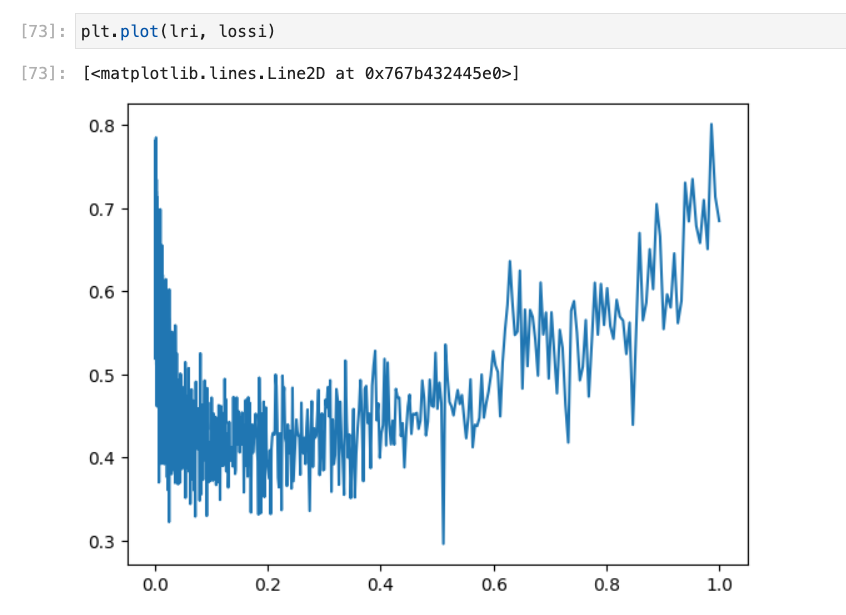
  or see from the exponent figure as below ( lri.append(lre[i])), we can see -1 exponent is a good choice.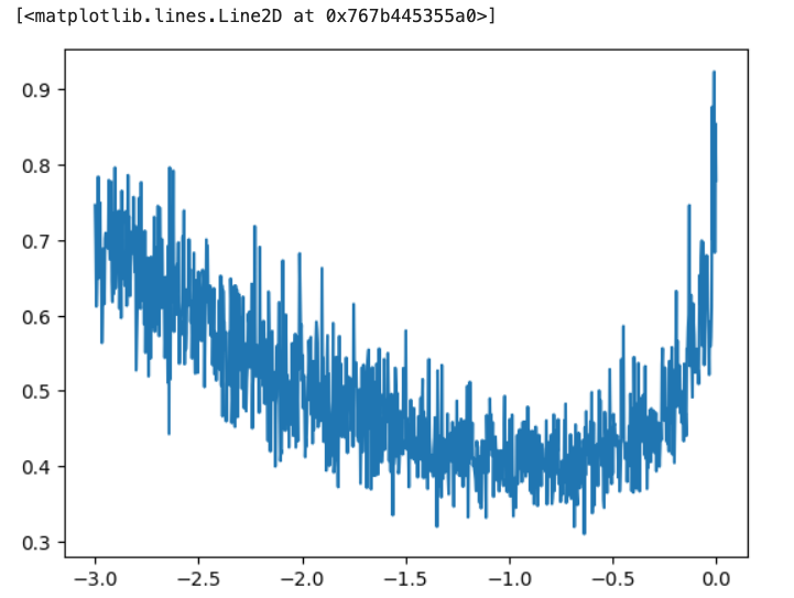

• Train/Vali/Test split
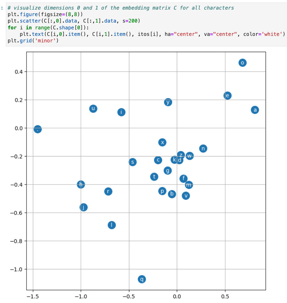
  80% - 10% - 10%

  import random
  random.seed(42)
  random.shuffle(words)
  n1 = int(0.8*len(words))
  n2 = int(0.9*len(words))
  
  Xtr, Ytr = build_dataset(words[:n1])
  Xdev, Ydev = build_dataset(words[n1:n2])
  Xte, Yte = build_dataset(words[n2:])
  

• Embedding visualization tensor.data: return the tensor tensor.item: return the scalar

4 Inference

# Get the prob from softmax
probs = F.softmax(logits, dim=1)
# Sample from the prob
ix = torch.multinomial(probs, num_samples=1, generator=g).item()
# crop and append
context = context[1:] + [ix]
# Save the generated ch to output
out.append(ix)