RL 2024-2

Focus on Policy Gradient in this post from Cameron Wolfe. 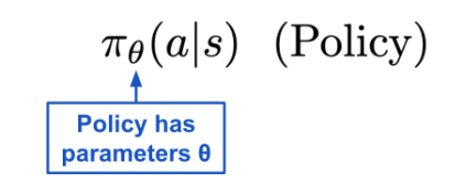and with implementation from Spinning up, it’s essencially a feedforward network (MLP with 3 layers in this example) with categorical output over action space.

# make core of policy network
# MLP input obs_dim and output n_acts
logits_net = mlp(sizes=[obs_dim]+hidden_sizes+[n_acts])

# make function to compute action distribution
def get_policy(obs):
    logits = logits_net(obs)
    return Categorical(logits=logits)

Couple of concepts to declarify Discount factor is necessary mathematically for infinate-horizon return Optimal value/Q functions here are all OFF-policy, silimiar to Q-learning.

1 Policy Optimization

The object function, or the loss function for policy gradient is here 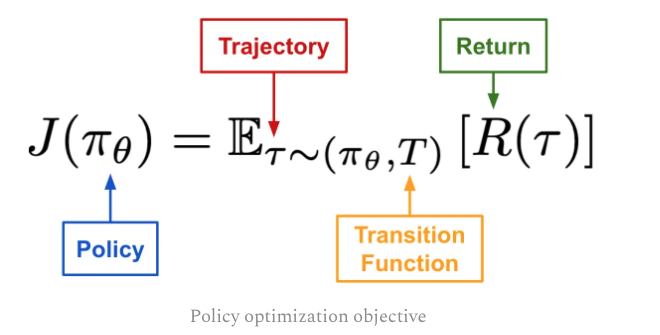and we can use GD if we can find the gradient of the object/loss function. 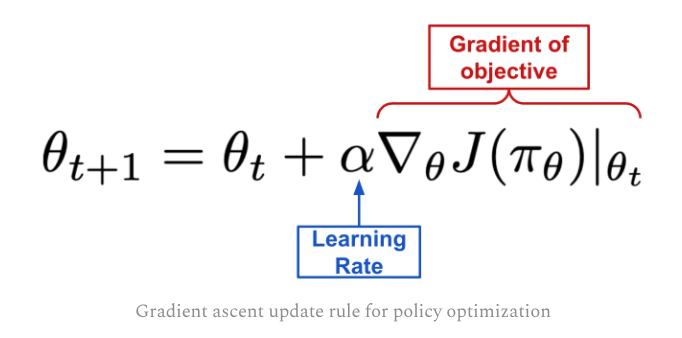To get the gradient, we need to see the object/loss function in integral or summation form 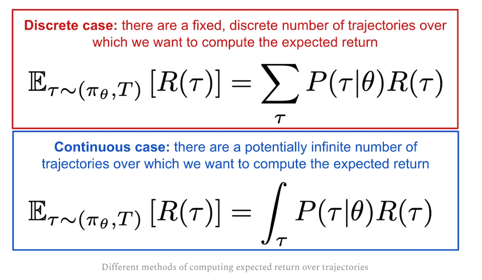and the trajectory prob. 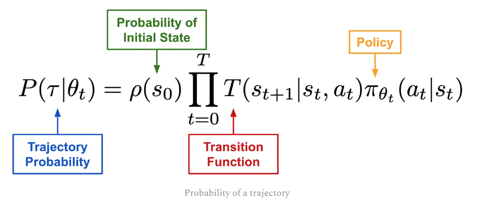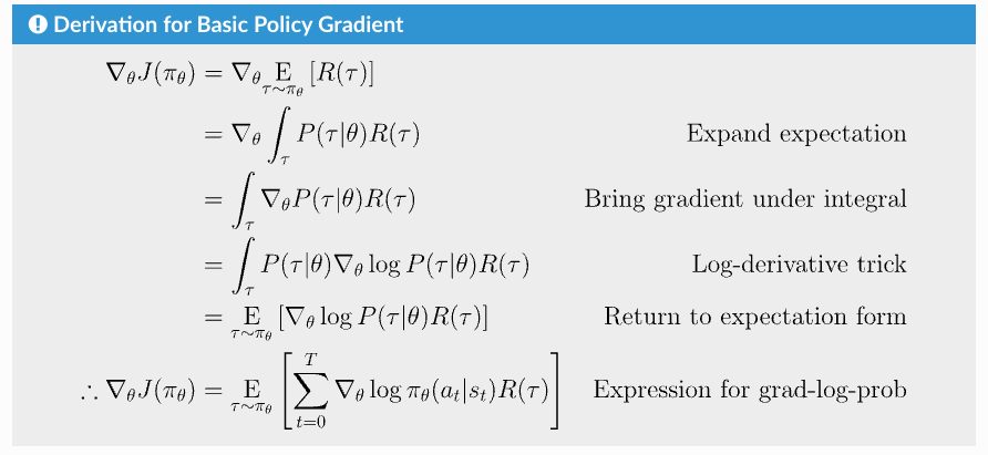P can be write out as following: Due to initial state and transition function are all independent of $\theta$,so only the gradient of policy is left 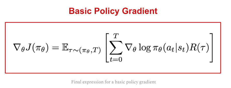Full derivation can be found here and summarized as below and it’s very simple in code. The loss here is VERY different from the loss in other ML. and it doesn NOT meansure performance

# make loss function whose gradient, for the right data, is policy gradient
def compute_loss(obs, act, weights):
    logp = get_policy(obs).log_prob(act)
    return -(logp * weights).mean()

# the weight for each logprob(a|s) is R(tau), same for every action
batch_weights += [ep_ret] * ep_len

2 Variants of Basic Policy Gradient

Only consider rewards after the current action, we have “reward-to-go” PG. It does NOT change the expected value of the PG but reduced the variance, so less trajectories required. 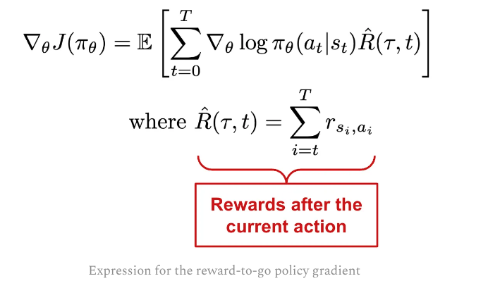The code change is only for the weights

def reward_to_go(rews):
    n = len(rews)
    rtgs = np.zeros_like(rews)
    for i in reversed(range(n)):
        rtgs[i] = rews[i] + (rtgs[i+1] if i+1 < n else 0)
    return rtgs
# the weight for each logprob(a_t|s_t) is reward-to-go from t
batch_weights += list(reward_to_go(ep_rews))

Adding a baseline, which only depends on $s_i$ to reward-to-go. It can use on-policy value function, which is the expected return from current state according to current policy. So this way will ONLY positively reinforce the trajectories (greater than the baseline)

This brings us Vanilla Policy Gradient.

Policy gradients are commonly formulated with the advantage function in RL, and various techniques have been proposed for deriving estimates of the advantage function. One of the most widely-used techniques is Generalized Advantage Estimation (GAE) may discuss later. This paper is from John Schulman and Philipp Moritz!