Spline

I reviewed some basics about Spline in the previous blog about KAN, and happened to find this tutorial. The most amazing part of this video is to show you what the Spline (wood strip) looks like originally, and how it worked!
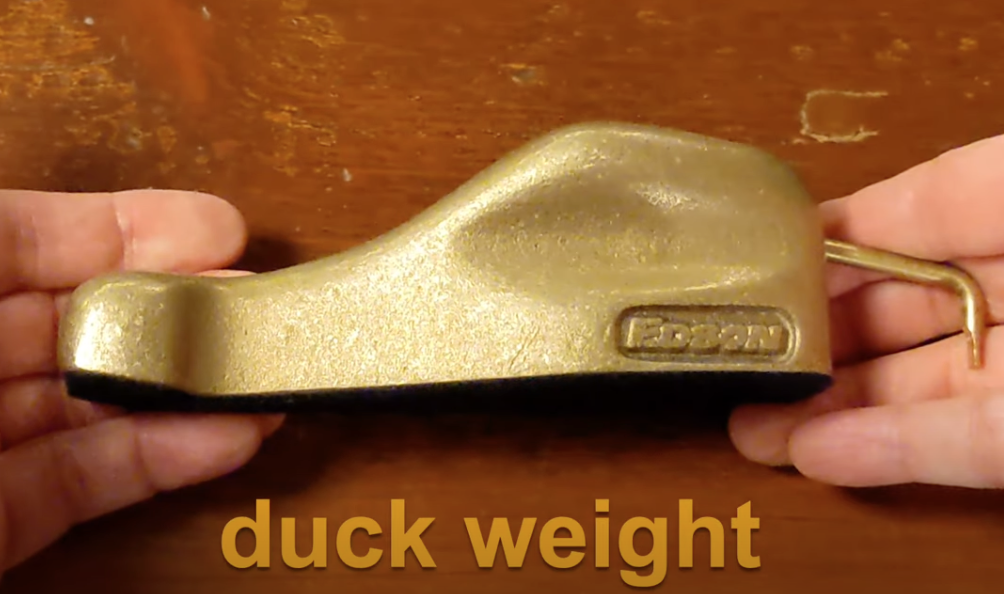
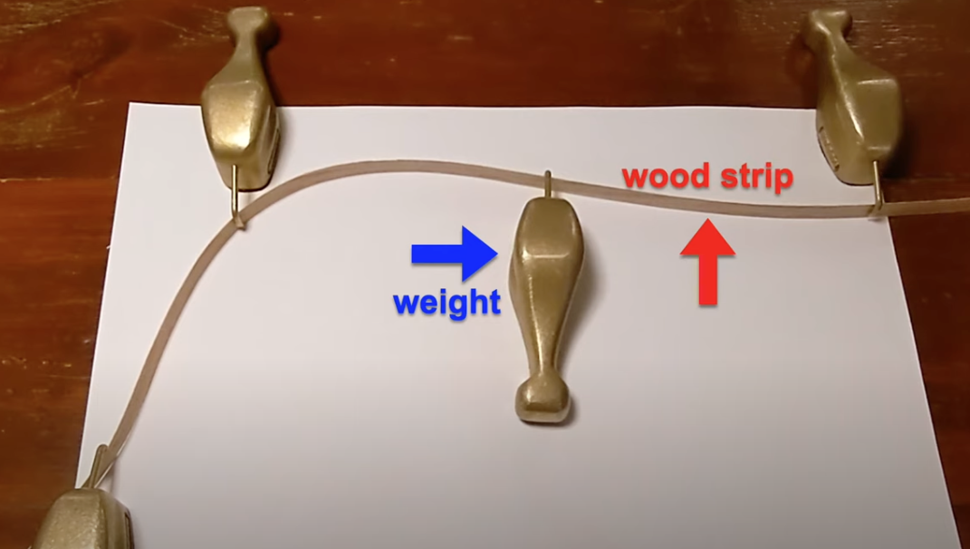and the weights used here are called duck weights, b/c they looks like duck head.

1 The intuition

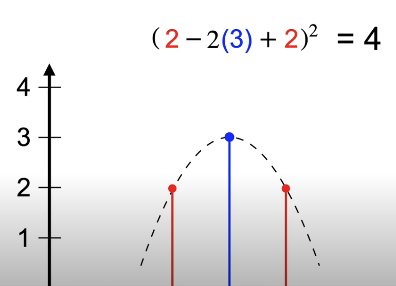
With the weights and wood strips setup as above, the natural force make the strip to bend following the rule to minimize bending energy, which mathamatically is the square of the second derivatives. Use 3 consective points as an example, \(E_{bend} = (f^{''})^2 \\= [f(t+1)-f(t)-(f(t)-f(t-1))]^2\)

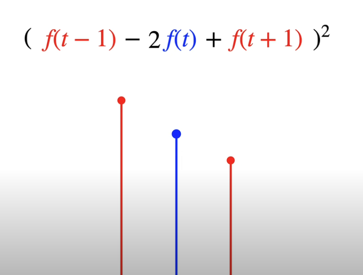
So when line is straight, bending energy is 0, otherwise, it’s greater than zero.

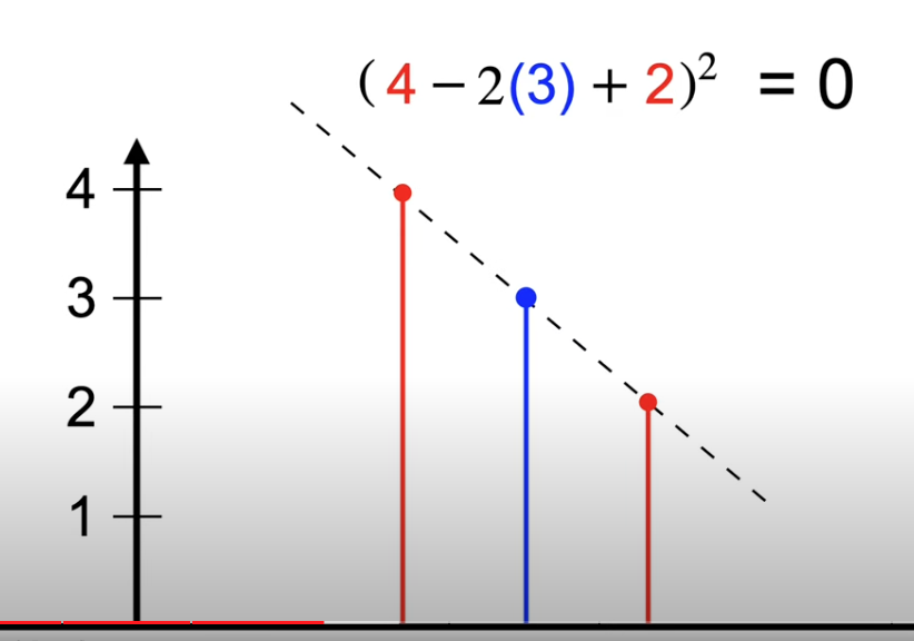
If we found a curve minimized the bending energy, it’s in the form of natural cubic spline, which is the shape wood strip bend naturally. How does it happens?

The part 3 uses a bee fly as an example, and the spline is the path of the bee. So the 2nd derivatly is the linked to accerlration and eventually the force.

\[min\int(\frac{d^2f}{dt^2})^2\\=min\int{a^2}=min\int{F^2}\]

What a beauty that minimum energy rule shows up here:)

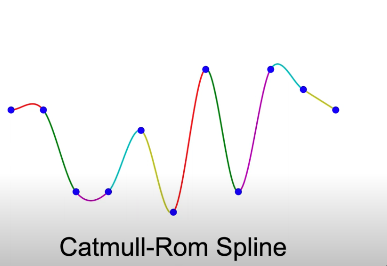
2 Catmull-Rom Spline

Spline is about concatencate polynomial together. The first derivative at the knot is the key factor to consider.
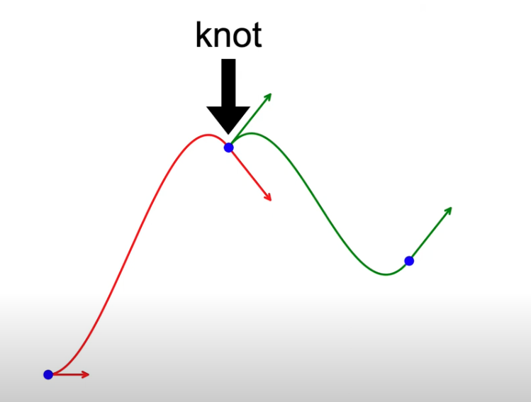
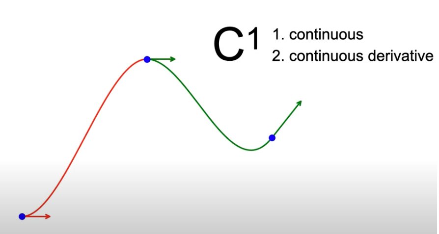
Making two derivatives the same would give you a $C_1$ smooth connection What should be the values of the two derivaties? Making it the same as the derivate of the two neighbor points is a no-brainer. 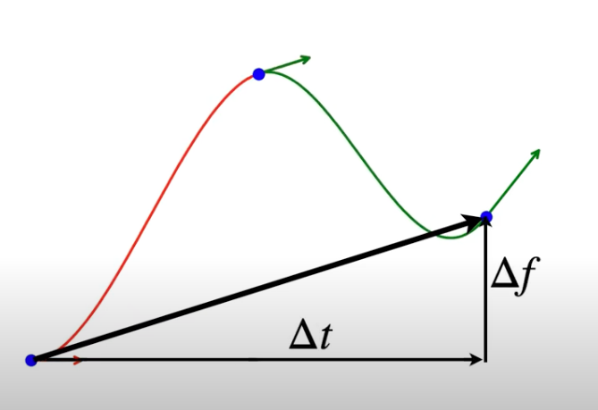and this gives you Catmull-Rom Spline.

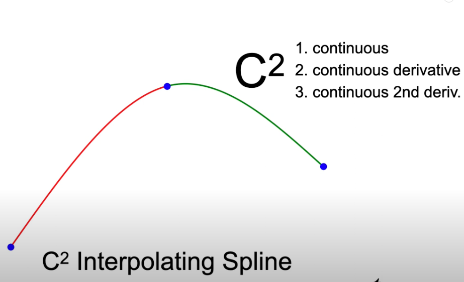
3 Natural Cubic Spline

Let’s change the contrains for a cubic spline with $n$ segments and It’s have $4n$ parameters to solve.
From control points perspective, each segments come with beg and end points, so total you will get $2n$ equations.
For $C_1$ continuous, you will get $n-1$ equations
For $C_2$ continuous, you will get $n-1$ equations
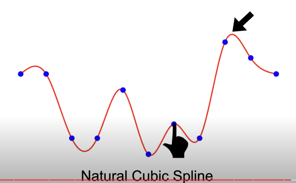
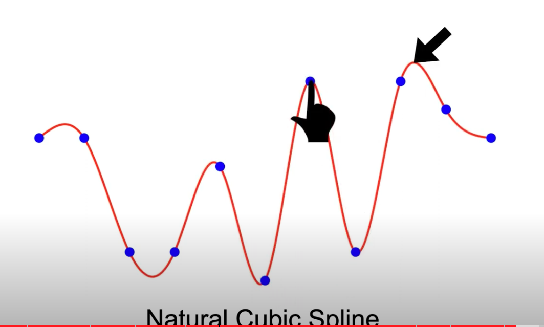
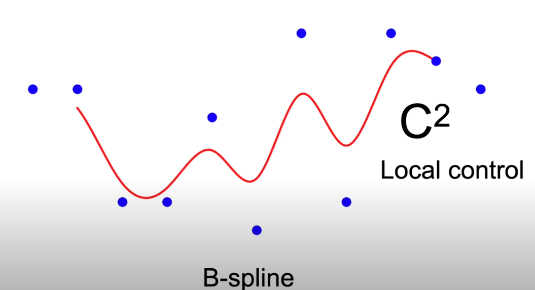
The last two constrains comes from forcing 2nd derivative of first and last points to be zero. Then we can get a special $C_2$ interpolating spline, natural cubic spline. The interpolation here means it goes through every control points. If we move one control points, if all other segments’s polynomial keeps the same, we call it local control, which feature natural cubic spline does NOT have.

4 B-Spline

In order to get a spline with $C_2$ continuity and local control, we introduce B-Spline, which does NOT have interpolation feature. The construction of B-spline is using Bezier Curve, which is always contained in the convex hull of the control points
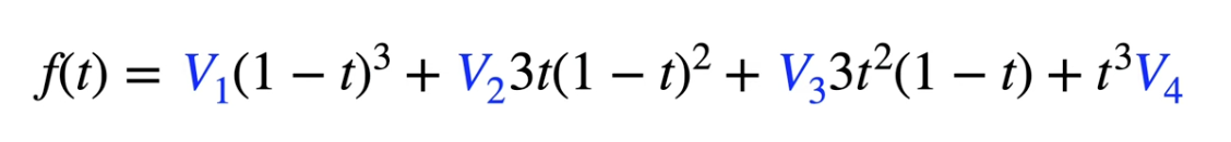
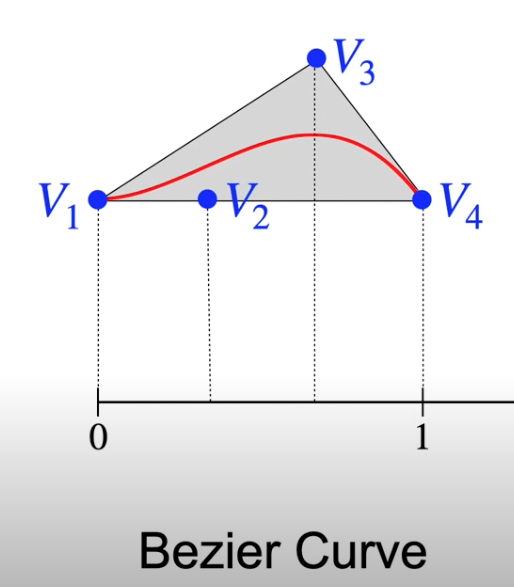and the curve can be directly written by the control points WITHOUT coefficients
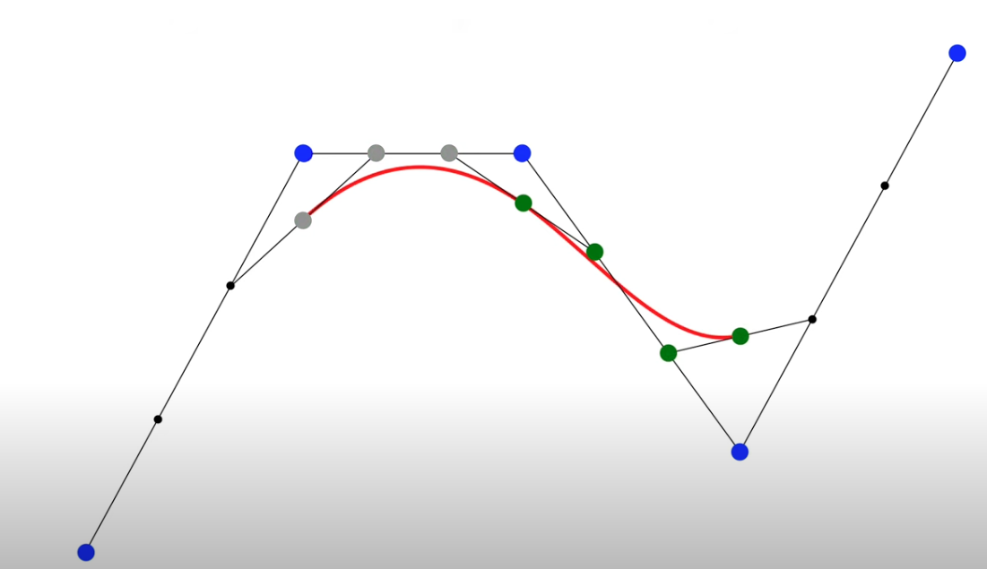
Here is the constructions of B-spline using Bezier curves

1. Start w first four control points and divide all segments into thirds
2. Connect the 1/3 points around the two center control points, and divide them by half
3. Use these 4 points to construct Bezier curve
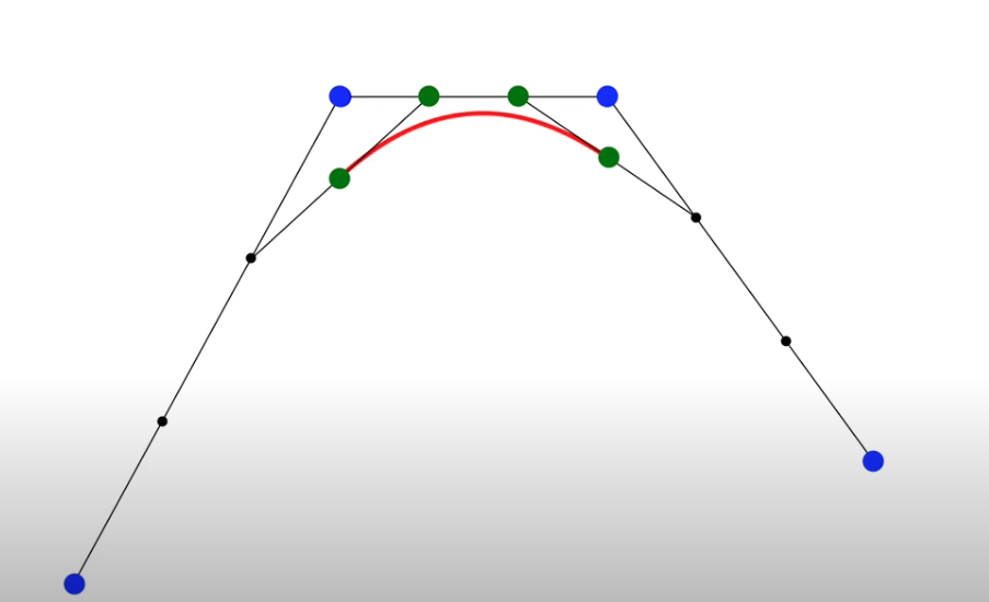
4. Now you can add a new control points and get a new Bezier curve.

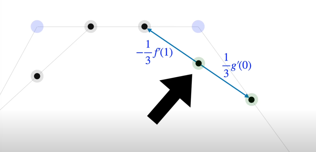
The two Bezier curves, f(x) and g(x) are both $C_1$ and $C_2$. THe proof of $C1$ is as follow b/c the derivaties are from the SAME line. $C_2$ approved is similar but didn’t show in the video :(

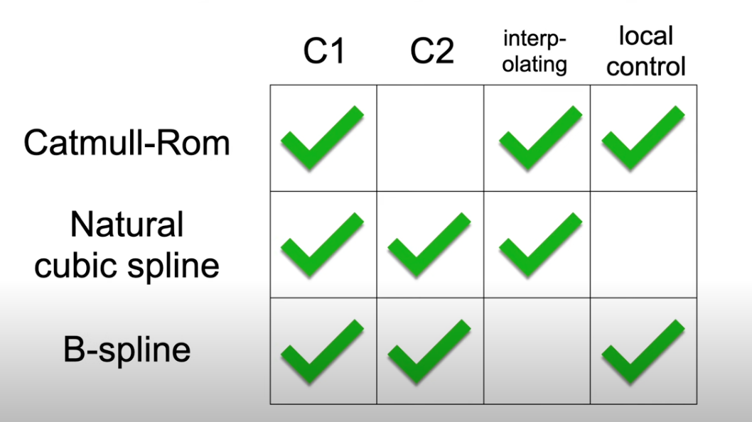
5 Summary

Here we summarize the 3 splines as below

2D splines are actually doing 2 1-D spline. Nothing specially. So skipped here.