Flow and Diffusion models Lab 1 (and Jupyter installation)

Reviewed the diffusion courses and take notes for Lab1

0 Jupyterlab on Mac and add Kernel in JupyterLab

1. Install Juypyter in Mac by brew install jupyterlab
2. Start Jupyter server by brew services start jupyterlab
3. Create a virtual env and activate it, install pip install ipykernel
4. In the venv, python -m ipykernel install --user --name my_env_name --display-name "My Custom Environment"
5. Now you should be able to see kernel My Custom Environment in Jupyter
6. Jupyter URL http://localhost:8888/lab

1 ODE and SED numerical methods

For Euler and Euler Maruyama methods

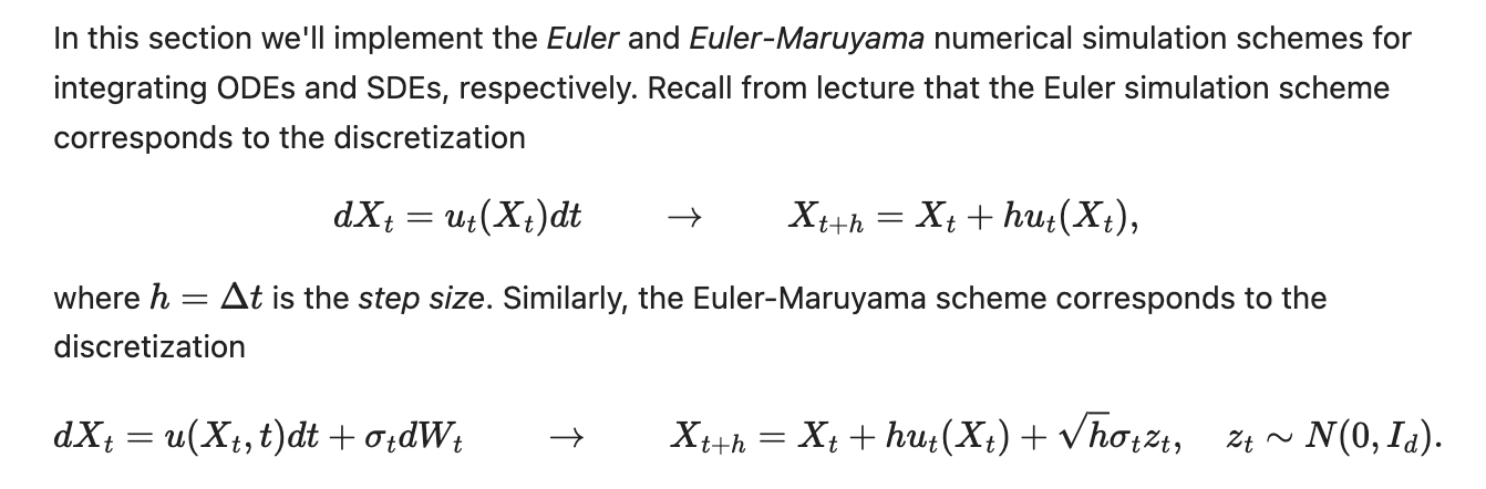
class EulerSimulator(Simulator):
    def __init__(self, ode: ODE):
        self.ode = ode
    def step(self, xt: torch.Tensor, t: torch.Tensor, h: torch.Tensor):
        return xt + self.ode.drift_coefficient(xt,t) * h
class EulerMaruyamaSimulator(Simulator):
    def __init__(self, sde: SDE):
        self.sde = sde
    def step(self, xt: torch.Tensor, t: torch.Tensor, h: torch.Tensor):
        return xt + self.sde.drift_coefficient(xt,t) * h + self.sde.diffusion_coefficient(xt,t) * torch.sqrt(h) * torch.randn_like(xt)

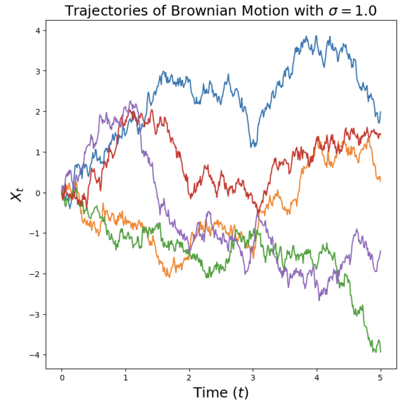
2 Brownian Motion for points

For Brownian motion is setting $u_t=0$ and $\sigma_t=\sigma$, viz., \(dX_t = \sigma dW_t, \quad \quad X_0 = 0.\)

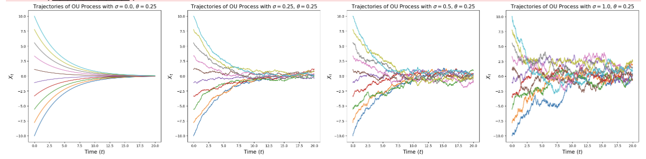
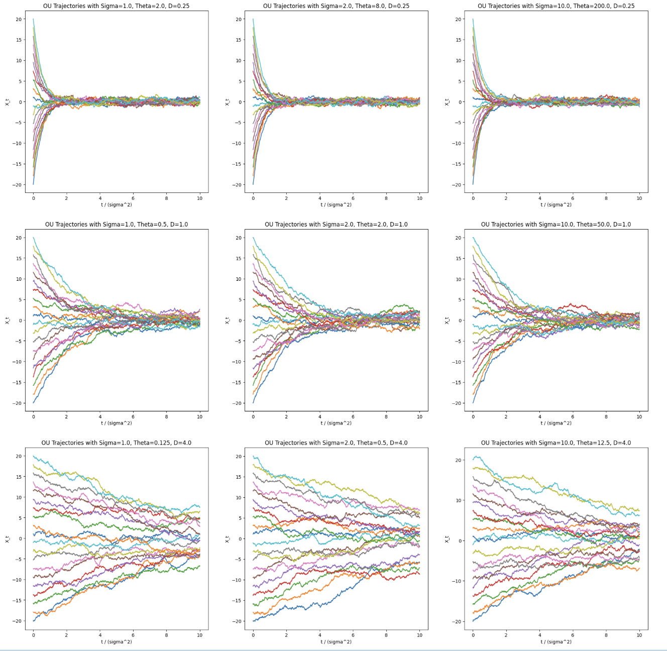
3 Ornstein-Uhlenbeck Process for points

An OU process is given by setting $u_t(X_t)=-{\theta}X_t$ and $\sigma_t=\sigma$, viz \(dX_t = -\theta X_t\,dt + \sigma\, dW_t, \quad \quad X_0 = x_0.\)

class OUProcess(SDE):
    def __init__(self, theta: float, sigma: float):
        self.theta = theta
        self.sigma = sigma
    def drift_coefficient(self, xt: torch.Tensor, t: torch.Tensor) -> torch.Tensor:
        """
        Returns the drift coefficient of the ODE.
        Args:
            - xt: state at time t, shape (bs, dim)
            - t: time, shape ()
        Returns:
            - drift: shape (bs, dim)
        """
        return - self.theta * xt
    def diffusion_coefficient(self, xt: torch.Tensor, t: torch.Tensor) -> torch.Tensor:
        return self.sigma * torch.ones_like(xt)

By fixing $D=\frac{\sigma^2}{2*\theta}$, you will get same images

4 Transform distributions

First, let’s define some distributions to play around with.

• The first quality is that one can measure the density of a distribution, which is the score $\nabla{\log{p(x)}}$.
• The second quality is that we can draw samples from the distribution.
  Here are 3 basic examples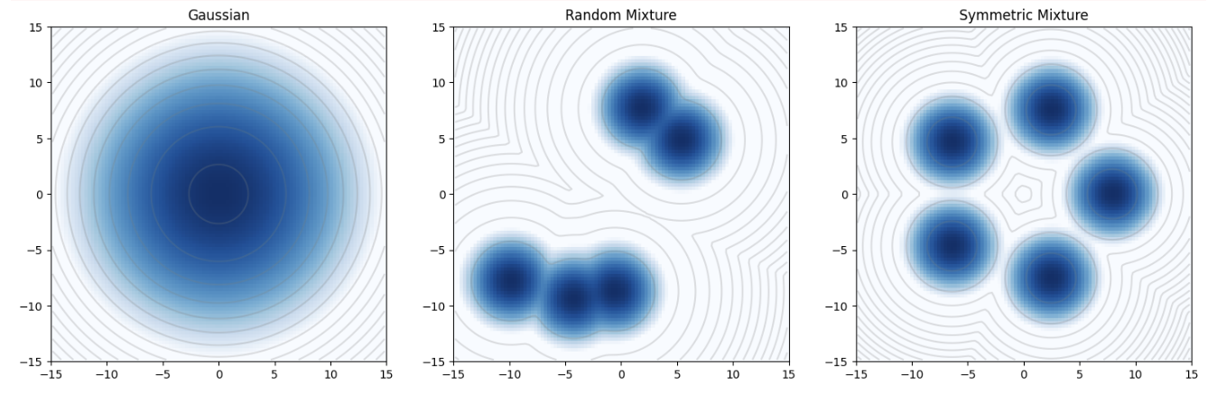

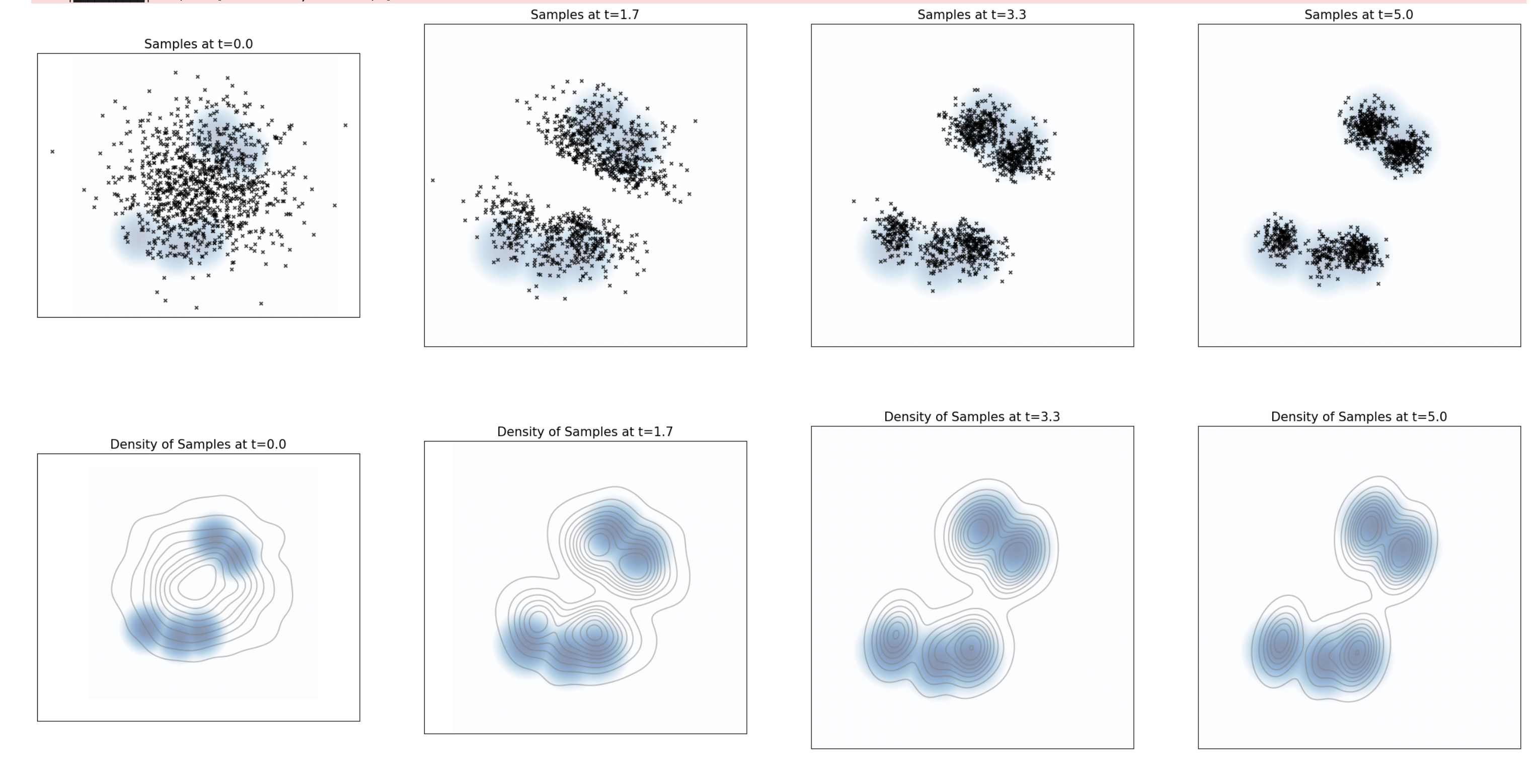
5 Langevin Dynamic

Here is the implementation of Langevin Dynamics \(dX_t = \frac{1}{2} \sigma^2\nabla \log p(X_t) dt + \sigma dW_t,\)

class LangevinSDE(SDE):
    def __init__(self, sigma: float, density: Density):
        self.sigma = sigma
        self.density = density # one of the sample distributions 
    def drift_coefficient(self, xt: torch.Tensor, t: torch.Tensor) -> torch.Tensor:
        """
        Returns the drift coefficient of the ODE.
        Args:
            - xt: state at time t, shape (bs, dim)
            - t: time, shape ()
        Returns:
            - drift: shape (bs, dim)
        """
        return 0.5 * self.sigma ** 2 * self.density.score(xt)
    def diffusion_coefficient(self, xt: torch.Tensor, t: torch.Tensor) -> torch.Tensor:
        """
        Returns the diffusion coefficient of the ODE.
        Returns:
            - diffusion: shape (bs, dim)
        """
        return self.sigma * torch.ones_like(xt)